A Simple & Essential Introduction To Graphs

A short, easy, but essential introduction to Graphs to help you ace them.

Graphs are extensively used in modern systems and applications.

• Social media networks like LinkedIn and Facebook use them to model people and their relationships to others.

• Search engines like Google use them as Knowledge Graphs to compile factual information.

• Platforms like Netflix and Spotify use them to build Recommendation systems.

• Package managers pip and npm use them for dependency management.

• Banks use them in their fraud detection algorithms.

• Google Maps uses them for efficient navigation and routing.

• They are used as Graph neural networks for drug discovery and protein analysis.

• LLMs use them for better information retrieval during response generation in a system called GraphRAG.

If you’re a software or ML engineer, you will most probably work with them during your career.

Here is a short, easy, but essential introduction to Graphs to help you ace them.

---

What is a Graph?

A Graph is a data structure that has two main components:

• Vertices or Nodes: that represent individual data points

• Edges: Connections between the Vertices or Nodes

For example, in a graph representing a social network, the vertices are individuals, and the edges represent relationships between them (friendship, spousal, etc.).

Graph visualised (Image from author’s book titled “Computer Science In 100 Images”)

A graph can be classified into different types based on multiple characteristics.

1. Based on Direction

• Directed graph
  In this type of graph, edges have a direction that indicates the flow of the relationship between the vertices they connect.
  For example, follower connections on Twitter, where a user follows another user in a one-way relationship.

• Undirected graph: Edges do not have direction in this type of graph, and connections go both ways.
  For example, a Facebook friend connection that connects two individuals who are friends.

2. Based on Edge Weights

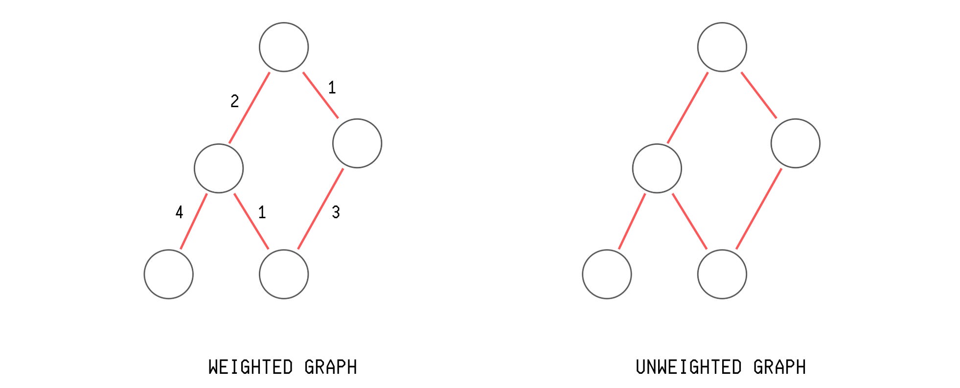
• Weighted graph
  Edges in this type of graph have a weight associated with them, which tells the strength of the relationship between vertices.
  For example, edge weights in a social network graph can represent the number of times two individuals communicate in a day.

• Non-weighted graph
  All edges are equally weighted in this type of graph, representing only the presence or absence of a relationship.
  For example, a graph of individuals related by the music they listen to.

3. Based on the Presence of Cycles

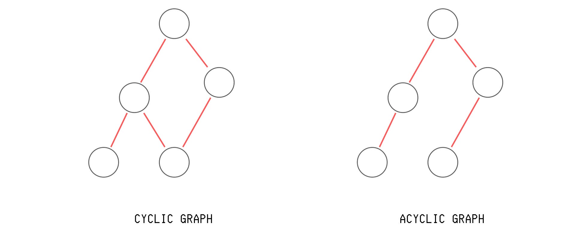
• Cyclic graph
  Loops exist between graph vertices in this type of graph. For example, a graph representing road networks in cities with roundabouts.

• Acyclic graph
  No loops exist between the graph vertices in this type of graph.

4. Based on the Connectivity Between All Vertices

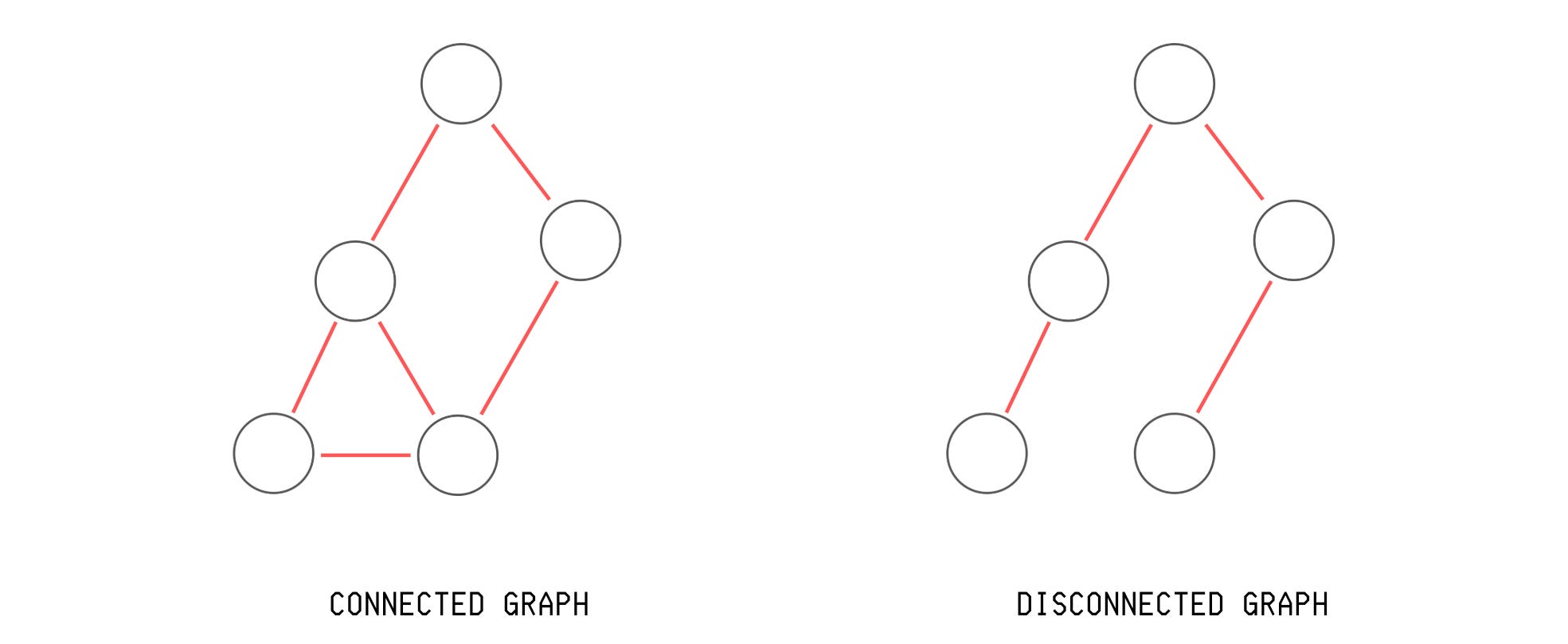
• Connected graph
  A path between every pair of vertices in this type of graph.
  For example, a graph representing a subway network within a single city.

• Disconnected graph
  There is at least one pair of vertices for which no path exists between them in this type of graph.

Apart from these, there are three other graph types that you might encounter and must know about.

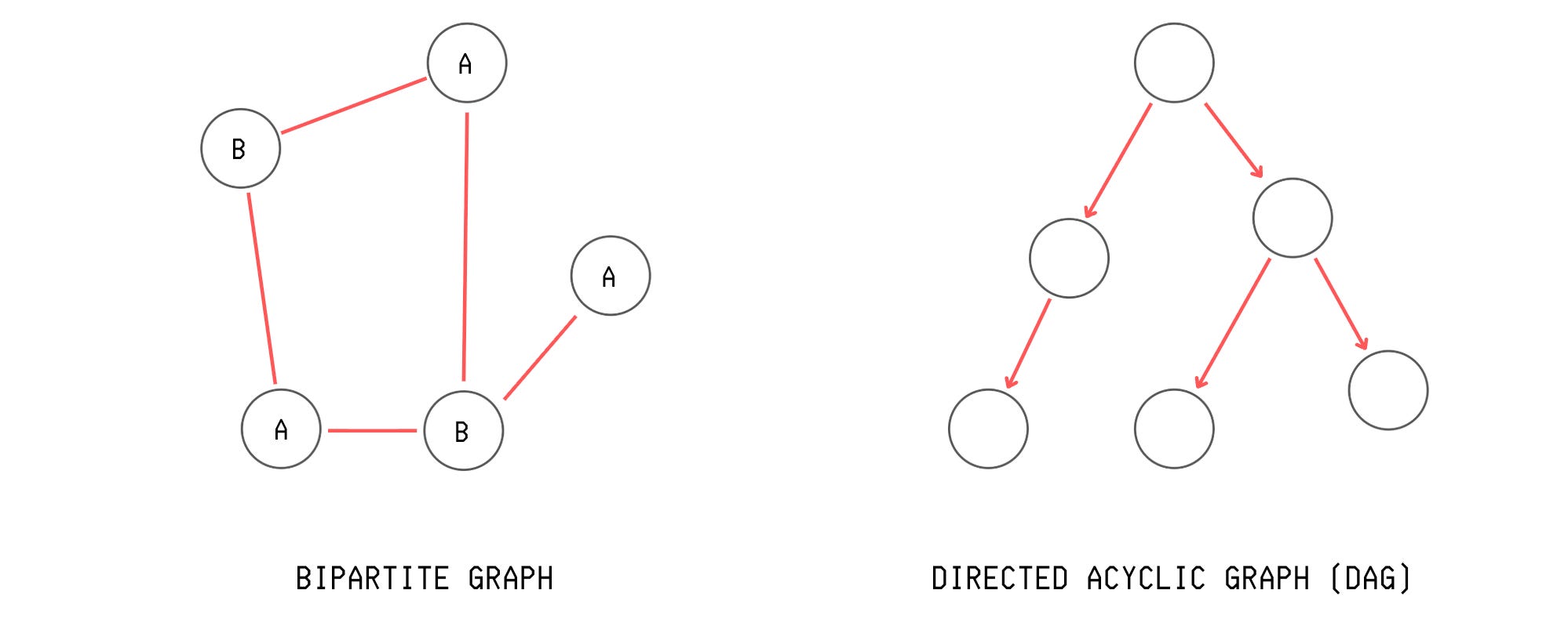
1. Directed Acyclic Graph (DAG): A directed graph that has no cycles.

   
   Use case: Neural network computation graphs in PyTorch and Git version control use a DAG.

2. Tree: A connected, acyclic, undirected graph where there is only one path between any two vertices.

   
   Use case: An Abstract Syntax Tree is used to represent the structure of a program or code snippet.

While DAGs can have multiple paths to the same vertex, a Tree is a type of DAG where there is only one path from root to any vertex.

3. Bipartite Graph: A graph where we can split the vertices into two groups, and each edge connects one vertex from one group to a vertex from the other group. There are no edges between vertices within the same group, as shown below.

   
   Use case: Recommendation systems are built using a bipartite graph to model the relationship between users and their preferred items.

---

How to Represent a Graph as a Data Structure

Let’s say we have an undirected, unweighted graph with four vertices A, B, C and D, and the following edges between them:

• A to B

• A to C

• A to D

• B to D

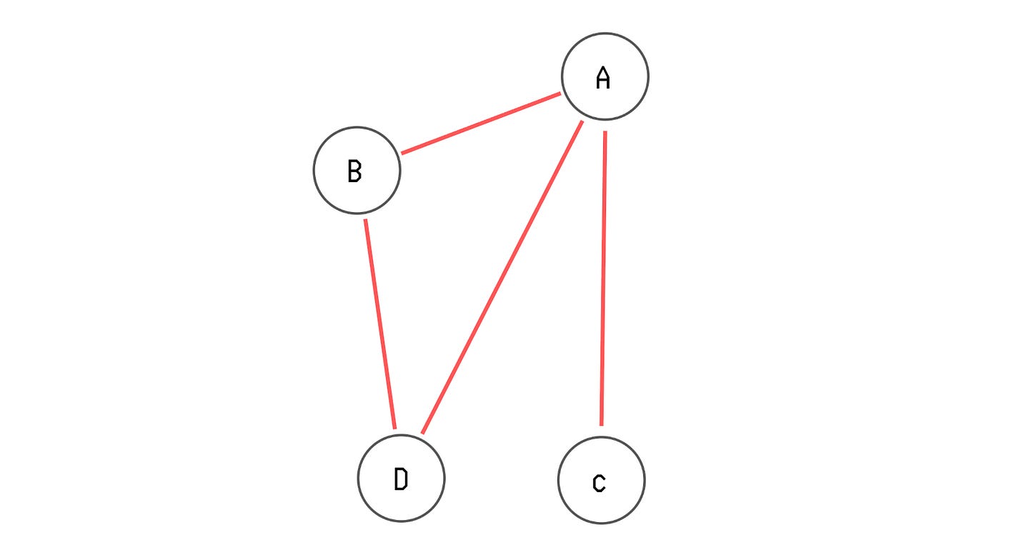
There are three ways to represent this graph.

1. Adjacency List: A data structure used to represent a graph, where each vertex in the graph stores an unordered array/ list of its neighboring vertices.

Advantage: It is a space-efficient way of storing sparse graphs. It is also easy to use with graph traversal algorithms, which we will discuss in the next section.

We can use the following Python data structures to build an adjacency list.

# Using list of lists
adj_list = [
    [’B’, ‘C’, ‘D’],  # neighbors of A (index 0)
    [’A’, ‘D’],       # neighbors of B (index 1)
    [’A’],            # neighbors of C (index 2)
    [’A’, ‘B’]        # neighbors of D (index 3)
]

# Using a dictionary
adj_list = {
    ‘A’: [’B’, ‘C’, ‘D’], # A connects to B, C, D
    ‘B’: [’A’, ‘D’],      # B connects to A, D
    ‘C’: [’A’],           # C connects to A
    ‘D’: [’A’, ‘B’]       # D connects to A, B
}

For weighted graphs, we can create an adjacency list as follows.

# Weighted graph using list of lists
# Index 1 in each tuple represents edge weight
weighted_graph_adj_list = [
    [(’B’, 4), (’C’, 2), (’D’, 7)], # neighbors and weights of A
    [(’A’, 4), (’D’, 5)],           # neighbors and weights of B
    [(’A’, 2)],                     # neighbors and weights of C
    [(’A’, 7), (’B’, 5)]            # neighbors and weights of D
]

# Weighted graph using dictionary 
# Index 1 in each tuple represents edge weight
weighted_graph_adj_list = {
    ‘A’: [(’B’, 4), (’C’, 2), (’D’, 7)], # A connects to B, C, D
    ‘B’: [(’A’, 4), (’D’, 5)],           # B connects to A, D
    ‘C’: [(’A’, 2)],                     # C connects to A
    ‘D’: [(’A’, 7), (’B’, 5)]            # D connects to A, B
}

2. Adjacency Matrix: A square matrix used to represent a graph, where the rows and columns correspond to the graph’s vertices.

In the following matrix, adj_matrix[i][j] (where i is the row and j is the column of the matrix) shows whether vertex i is connected to vertex j.

A value of 1 indicates a connection, and 0 means no connection.

Advantage: It is used to store dense graphs, and makes it easy to check if two vertices are connected in constant or O(1) time by accessing adj_matrix[i][j].

It is also used in the Floyd-Warshall algorithm to efficiently compute the shortest paths between all pairs of vertices in a dense graph.

We can create an adjacency matrix in Python as follows.

# Using list of lists
adj_matrix = [
    [0, 1, 1, 1],  # A: B, C, D
    [1, 0, 0, 1],  # B: A, D
    [1, 0, 0, 0],  # C: A
    [1, 1, 0, 0],  # D: A, B
]

For a weighted graph, an adjacency matrix is created in Python as follows.

# Using list of lists
weighted_graph_adj_matrix = [
    [0, 4, 2, 7],  # Weights from A to A,B,C,D
    [4, 0, 0, 5],  # Weights from B to A,B,C,D
    [2, 0, 0, 0],  # Weights from C to A,B,C,D
    [7, 5, 0, 0]   # Weights from D to A,B,C,D
]

3. Edge list: A data structure used to represent a graph as a list of its edges.

Advantage: It is the easiest format to read, parse, and generate. It is used in algorithms focused on edges rather than vertices, such as Kruskal’s algorithm for finding a minimum spanning tree.

We can create an edge list in Python as follows.

# Using a list of tuples
edge_list = [
    (’A’, ‘B’), (’A’, ‘C’), (’A’, ‘D’),
    (’B’, ‘A’), (’B’, ‘D’),
    (’C’, ‘A’),
    (’D’, ‘A’), (’D’, ‘B’)
]

# Using a list of lists
edge_list = [
    [’A’, ‘B’], [’A’, ‘C’], [’A’, ‘D’],
    [’B’, ‘A’], [’B’, ‘D’],
    [’C’, ‘A’],
    [’D’, ‘A’], [’D’, ‘B’]
]

For weighted graphs, this is done as follows.

# Using a list of tuples with each tuple as (vertex_1, vertex_2, weight)
weighted_graph_edge_list = [
    (’A’, ‘B’, 4), (’A’, ‘C’, 2), (’A’, ‘D’, 7),
    (’B’, ‘A’, 4), (’B’, ‘D’, 5),
    (’C’, ‘A’, 2),
    (’D’, ‘A’, 7), (’D’, ‘B’, 5)
]

# Using a list of lists with each inner list as [vertex_1, vertex_2, weight]
weighted_graph_edge_list = [
    [’A’, ‘B’, 4], [’A’, ‘C’, 2], [’A’, ‘D’, 7],
    [’B’, ‘A’, 4], [’B’, ‘D’, 5],
    [’C’, ‘A’, 2],
    [’D’, ‘A’, 7], [’D’, ‘B’, 5]
]

---

How To Create A Graph In Python

The most common representation of a graph that you will commonly work with is an adjacency list in the form of a list of lists.

Let’s write a function called build_adjacency_list that helps create a graph as an adjacency list given a list of edges.

The parameters of the function are:

• n: Number of vertices in the graph

• edges : A list of edges where each edge is a list containing either two values representing the connected vertices for an unweighted graph, or three values representing the connected vertices and the edge weight for a weighted graph.

• directed : Whether the graph is directed.

• weighted: Whether the graph is weighted.

def build_adjacency_list(n, edges, directed=False, weighted=False):
    # Initialize adjacency list with n empty lists
    graph = [[] for _ in range(n)]
    
    # If edges have weights
    if weighted:
        # Iterate through each edge in the edge list
        for edge in edges:
            vertex_1, vertex_2, weight = edge[0], edge[1], edge[2]
            
            # Add weighted edge as a tuple to vertex_1’s list
            graph[vertex_1].append((vertex_2, weight))
            
            # For undirected graphs, add reverse edge as well
            if not directed:
                graph[vertex_2].append((vertex_1, weight))
    
    # If edges have no weights
    else:
        # Iterate through each edge in the edge list
        for edge in edges:
            vertex_1, vertex_2 = edge[0], edge[1]
            
            # Add vertex_2 to vertex_1’s adjacency list
            graph[vertex_1].append(vertex_2)
            
            # For undirected graphs, add reverse edge as well
            if not directed:
                graph[vertex_2].append(vertex_1)
    
    return graph

Given four vertices (0 to 3) and a list of edges between them (Edge list), the adjacency list created using this function is as follows.

edges = [[0, 1], [0, 2], [0, 3], [1, 3]]

build_adjacency_list(4, edges)
# [[1, 2, 3], [0, 3], [0], [0, 1]]

Next, to create an adjacency matrix, we can use the following function with the same parameters as described above.

def build_adjacency_matrix(n, edges, directed=False, weighted=False):
    # Initialize an n x n matrix filled with zeros
    matrix = [[0] * n for _ in range(n)]

    # Iterate through each edge in the edge list
    for edge in edges:
        # Get weight if the graph is weighted, otherwise use 1 as default
        vertex_1, vertex_2, weight = (edge[0], edge[1], edge[2]) if weighted else (edge[0], edge[1], 1)
        
        # Set the weight for the edge from vertex_1 to vertex_2
        matrix[vertex_1][vertex_2] = weight

        # For undirected graphs, add reverse edge as well
        if not directed:
            matrix[vertex_2][vertex_1] = weight

    return matrix

An adjacency matrix created from the given edge list is as follows.

edges = [[0, 1], [0, 2], [0, 3], [1, 3]]

build_adjacency_matrix(4, edges)
# [[0, 1, 1, 1], [1, 0, 0, 1], [1, 0, 0, 0], [1, 1, 0, 0]]

---

How To Move Through A Graph?

There are two fundamental algorithms, called Graph Traversal Algorithms, that allow us to systematically explore a graph’s vertices. These are described as follows.

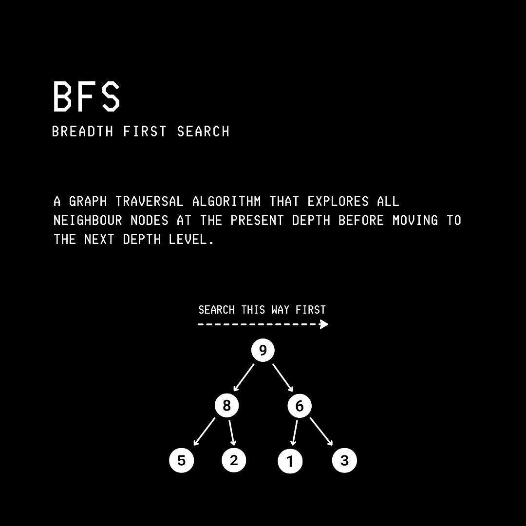
1. Breadth-First Search (BFS)

This is a graph traversal algorithm that explores a graph level by level, visiting a source vertex’s neighbors before going deeper.

Breadth-First Search (BFS) visualised (Image from author’s book titled “Computer Science In 100 Images”)

Let’s say that we are given the following graph.

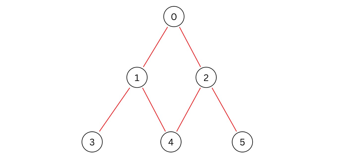
An adjacency list representation of this graph is as follows.

adj_list = [[1, 2], [3, 4], [4, 5], [], [], []]

We write and perform BFS over it using a Queue.

# Iterative method using a Queue (FIFO data structure)

def bfs(graph, start):
    “”“ 
    Params: 
        graph: adjacency list
        start: starting vertex
    “”“
    # Create empty set to store visited vertices
    visited = set()

    # Create queue using a list initialized with start vertex
    queue = [start]

    # Mark the starting vertex as visited
    visited.add(start)

    # Loop while there are vertices in the queue
    while queue:
        # Remove and get the first element from queue (FIFO)
        vertex = queue.pop(0)

        # Print the current vertex being processed
        print(vertex, end=” “)

        # Iterate through all neighbors of current vertex
        for neighbor in graph[vertex]:
            # Check if neighbor hasn’t been visited yet
            if neighbor not in visited:
                # Mark neighbor as visited
                visited.add(neighbor)

                # Add neighbor to the end of queue for processing later
                queue.append(neighbor)

# Perform BFS starting from vertex 0
bfs(adj_list, 0) # 0 1 2 3 4 5

2. Depth-First Search (DFS)

This is a graph traversal algorithm that explores a graph by following each path to its deepest point before backtracking and trying alternative paths.

Depth-First Search (DFS) visualised (Image from author’s book titled “Computer Science In 100 Images”)

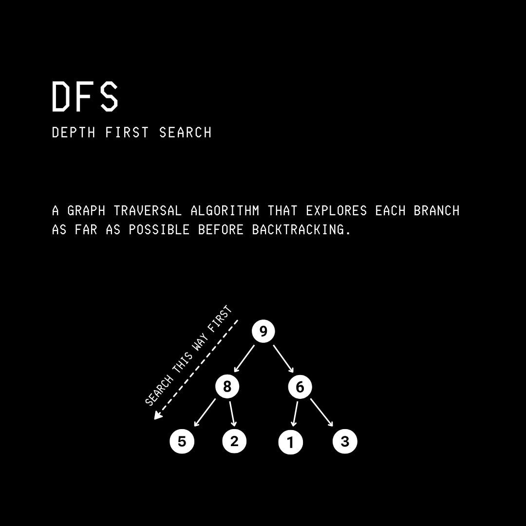
Going back to the graph and its adjacent list representation shown below:

adj_list = [[1, 2], [3, 4], [4, 5], [], [], []]

There are two ways we can write and perform DFS on it.

1. Using Recursion

def dfs_recursive(graph, start, visited=None): 
    “”“ 
    Params: 
        graph: adjacency list
        start: starting vertex
        visited: set of processed vertices
    “”“
    # Initialize visited set on first call
    if visited is None:
        visited = set()
    
    # Mark the current vertex as visited
    visited.add(start)
    
    # Print the current vertex being processed
    print(start, end=” “)
    
    # Iterate through all neighbors of current vertex
    for neighbor in graph[start]:
        # Check if neighbor hasn’t been visited yet
        if neighbor not in visited:
            # Recursively call DFS on the unvisited neighbor
            dfs_recursive(graph, neighbor, visited)

# Perform DFS recursively starting from vertex 0
dfs_recursive(adj_list, 0)  # 0 1 3 4 2 5

2. Using iteration with a Stack (LIFO data structure)

def dfs_iterative(graph, start):
    “”“ 
    Params: 
        graph: adjacency list
        start: starting vertex
    “”“
    # Create empty set to store visited vertices
    visited = set()
    
    # Create stack using a list initialized with start vertex
    stack = [start]

    # Loop while there are vertices in the stack
    while stack:
        # Remove and get the last element from stack
        vertex = stack.pop()
        
        # Check if vertex hasn’t been visited yet
        if vertex not in visited:
            # Print the current vertex being processed
            print(vertex, end=” “)
            
            # Mark the current vertex as visited
            visited.add(vertex)

            # Add neighbors in reverse so that left-most is processed first
            for neighbor in reversed(graph[vertex]):
                # Add neighbor to the top of stack for processing later
                stack.append(neighbor)

# Perform DFS iteratively starting from vertex 0
dfs_iterative(adj_list, 0) # 0 1 3 4 2 5

---

That’s everything for this lesson on graphs. If you loved reading it, consider sharing it with others.💚

It takes me a long time to write these valuable tutorials for you. If you want to support my work and get even more value from this publication, consider becoming a paid subscriber.

You can also check out my books on Gumroad and connect with me on LinkedIn to stay in touch.