Hierarchical Reasoning Model: A Deep Dive

A deep dive into the Hierarchical Reasoning Model to understand its internals that help it outperform powerful reasoning models available to us today.

Aug 10, 2025

Reasoning well is one of the biggest challenges for AI models available today.

Most popular LLMs use Chain-of-Thought (CoT) prompting and Inference time scaling for reasoning, but they still aren’t good enough.

Even with their imperfect reasoning approach, these models have very high latency and are too expensive for everyday use.

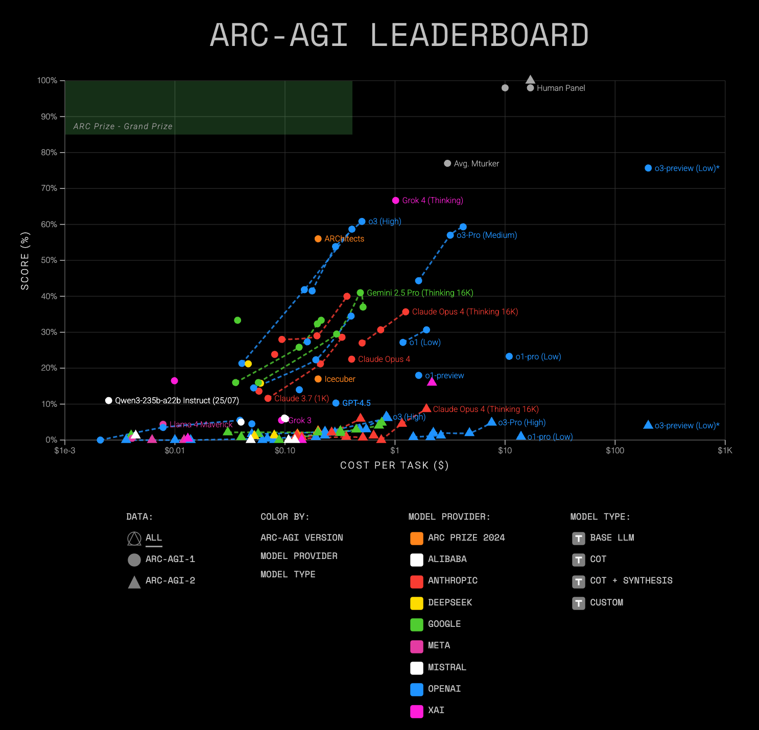
Check out the performance of the current most powerful LLMs on the ARC-AGI benchmarks, which contain tasks that are easy to solve for humans, yet hard, or impossible, for AI.

ARC-AGI benchmarks leaderboard (Source: Arc Prize)

But this is about to change.

A small Singapore-based AI lab, founded in 2024, called Sapient Intelligence, has just open-sourced and published a new AI architecture called Hierarchical Reasoning Model (HRM) that has shocked the AI community.

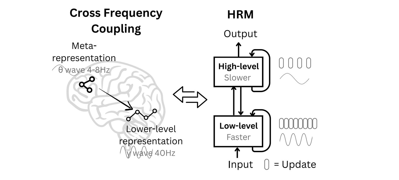
The HRM architecture is inspired by the human brain and uses two interdependent recurrent networks:

a slower, high-level module for abstract, deliberate reasoning (the “Controller” module)
a faster, low-level module for detailed computations (the “Worker” module)

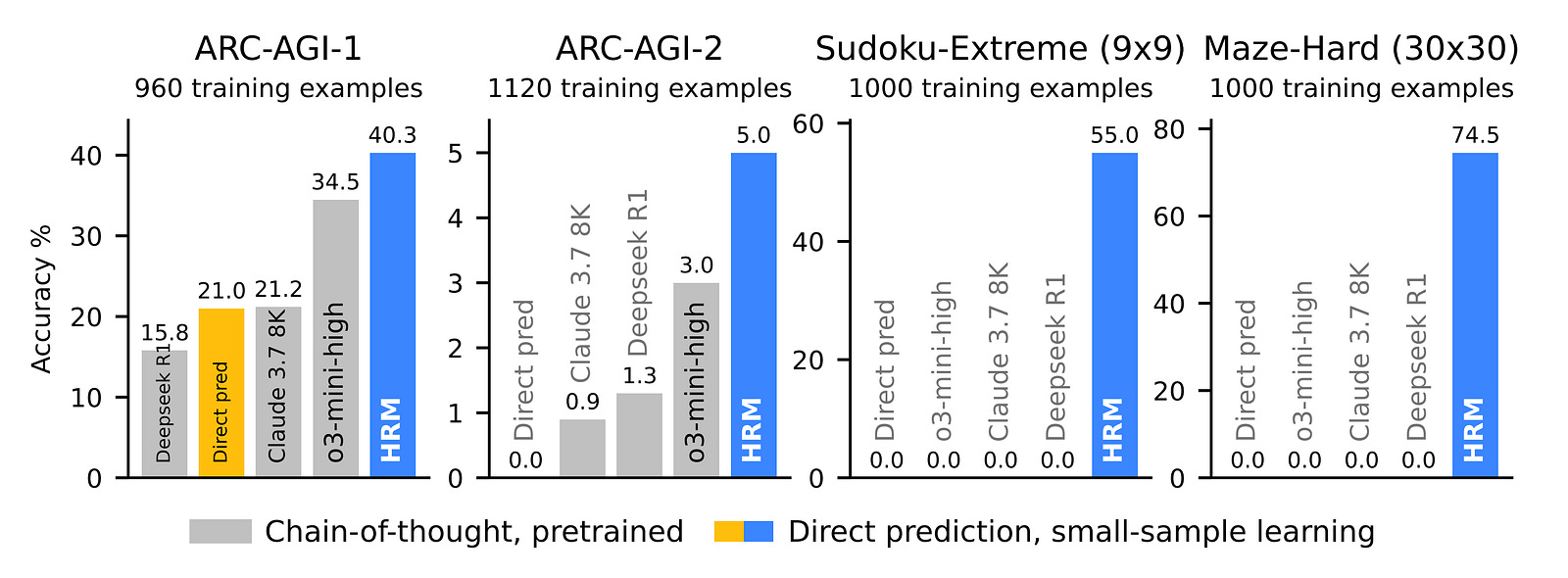
HRM uses two interdependent recurrent neural networks that work at different paces, mimicking how the brain processes information to solve problems.

With only 27 million parameters and only 1000 training samples, an HRM can achieve nearly perfect performance on complex Sudoku puzzles and optimal path finding challenges in large mazes.

In comparison, o3-mini-high, Claude 3.7 8K, and DeepSeek-R1 all have zero accuracy on this task.

Alongside this, an HRM outperforms all of these models on ARC-AGI-1 and ARC-AGI-2 benchmarks, directly from the inputs without any pre-training or CoT data.

HRM outperforms all other strong reasoning LLMs on complex Sudoku puzzles, optimal path finding in large mazes, and ARC-AGI benchmarks.

Here is a story where we deep dive into how a Hierarchical Reasoning Model works and understand its internals that help it outperform powerful reasoning models available to us today.

But First, Why Can’t Our Current LLMs Reason Well?

Deep neural networks are the backbone of all the Artificial Intelligence popularly available to us today.

Deep neural networks operate on a fundamental principle: the deeper a network (the more layers it has), the better it performs.

The most successful architecture, called Transformer, that powers all our LLMs is again a deep neural network that follows this principle.

However, there’s a problem: the LLM architecture is fixed, and its depth doesn't grow with the complexity of the problem being solved.

This makes them unsuitable for solving polynomial-time problems.

LLMs also aren’t Turing complete.

(Turing-complete systems can perform any computation that can be described by an algorithm as long as it has enough time and memory.)

To work around these limitations, LLMs rely on Chain-of-Thought (CoT) prompting, which is a technique of reasoning that breaks down complex tasks into simpler intermediate steps before solving them.

However, CoT prompting involves reasoning using human language. This is different from how humans do it. For humans, language is primarily a tool for communication rather than reasoning or thought.

This also means that a single misstep can lead to the reasoning derailing completely.

Furthermore, training reasoning LLMs requires a massive amount of long CoT data, which makes this process expensive, raising a concern about whether we will run out of data to train future LLMs on.

Alongside this, generating numerous tokens for complex reasoning tasks results in slow response times and increased use of computational resources at inference/ test time.

What Can We Learn About Reasoning From The Human Brain?

While LLMs use explicit natural language for reasoning, humans reason in a latent space without constant translation back and forth to language.

Following this insight, researchers from Meta published a technique called Chain of Continuous Thought (CoConuT) in 2024, which outperformed CoT in many logical reasoning tasks while using fewer reasoning tokens during inference.

Since then, many such techniques have been introduced, but they all suffer from a limitation.

The LLMs being trained for latent reasoning aren’t deep enough, as stacking up more and more layers leads to vanishing gradients, which means no learning for the model.

LLMs also use Backpropagation through time (BPPT), which is incompatible with research on how the human brain learns.

The next natural question from here is: So, how does the human brain really learn and reason?

We do not have a complete answer to this question, but we know that the brain is structured in layers or different levels, and these levels process information at different speeds.

The low-level regions react fast to sensory inputs like vision, and for movement, and the high-level regions are used for integrating information over longer timescales and slow computations, like abstract planning.

The slow, higher-level areas guide the fast, lower-level circuits that then execute a task. This is evident by different brain waves (slow theta waves and fast gamma waves).

Both areas also use feedback loops that help refine thoughts, change decisions, and learn from experience.

This hierarchical model in the brain gives it sufficient “computational depth” for solving challenging tasks.

Could we borrow these concepts and create an AI architecture that can replicate what we know about how the human brain works?

Here Comes ‘Hierarchical Reasoning Model’

Inspired by the human brain, the Hierarchical Reasoning Model (HRM) architecture consists of four components:

Input network (f(I))
Low-level recurrent module (L-module represented by f(L) or the “Worker” module)
High-level recurrent module (H-module represented by f(H) or the “Controller” module)
Output network (f(O))

An HRM performs reasoning over N high-level cycles, each containing T low-level timesteps. This makes the total timesteps per forward pass N × T.

The modules f(L) and f(H) each keep a hidden state z(i)(L) and z(i)(H) respectively (where i is the current timestep), which are initialized as z(0)(L) and z(0)(H).

Forward Pass In An HRM

Given an input x, it is first projected into a representation x̃ by the input network f(I).

At each timestep i, the low-level module (L-module) updates its state based on:

its previous state z(i-1)(L)
the high-level module’s current state z(i-1)(H) (which remains fixed throughout a cycle), and
the input representation x̃

The high-level module (H-module) only updates once at the end of each cycle, i.e., every T timesteps using the low-level or L-module’s final state at the end of that cycle.

After N full cycles (or N X T timesteps), a final prediction ŷ is extracted from the hidden state of the high-level module using the output network.

A halting mechanism (which we will discuss later) decides whether the model should end its processing and use ŷ as the final prediction, or proceed with another forward pass.

Alongside the halting mechanism, the HRM uses many specialized techniques that enable it to perform so well. Let’s discuss them next.

Hierarchical Convergence To Fix The Problem Of Early Convergence

Recurrent networks suffer from the problem of early convergence.

As training proceeds, their hidden state moves towards a fixed point, the update magnitudes shrink, and learning with each future step slows down to none.

A goal of researchers was, therefore, to slow this convergence process for effective learning in HRM.

This is done using a process called Hierarchical Convergence, which works as follows.

During each cycle with T timesteps, the L-module converges towards a local equilibrium based on the state of the H-module.

After a cycle is complete, the H-module performs its own update based on the final state of the L-module.

In the next cycle, the L-module uses this updated state of the H-module to reach a different local equilibrium. (Think of this as the L-module resetting with each cycle guided by the H-module.)

This process allows the H-module to function as a “Controller” that directs the overall problem-solving strategy, while the L-module functions as a “Worker” executing the refinement required at each step.

If this were a normal recurrent network, it would have converged in T timesteps. Instead, an HRM achieves stable and prolonged convergence over N x T timesteps, leading to better performance.

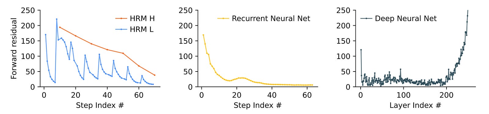
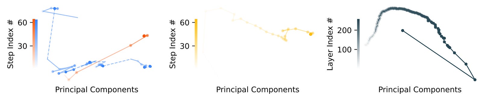
Plots showing the Forward residuals (difference between states across timesteps) at each time step in an HRM and RNN, and across layers in a DNN. In a standard RNN, the residuals drop quickly to zero, indicating early convergence. This is in contrast to HRM, where residuals show cyclic activity (L-module resets, H-module gradually converges). DNN shows vanishing gradients with the largest residuals (or learning) only in the initial and final layers.

PCA (Principal Component Analysis) is a technique that finds the directions (called principal components) along which a model’s hidden states vary the most.

The PCA analysis on different models is shown below.

PCA plots showing how the hidden state of the model evolves over time (for RNN/ HRM) or through layers (in DNN). The HRM explores rich representations across the time steps, the RNN quickly collapses into a fixed representation, and the DNN changes mainly at the input/output layers, while the middle layers suffer from vanishing gradients and little learning.

Avoiding Backpropagation By Approximating Gradients In One Step

Standard recurrent networks use Backpropagation to compute gradients, which requires them to store the hidden states from the forward pass and then combine them with gradients during the backward pass.

This requires O(T) memory (space complexity) for T steps. It also means that one has to keep batch sizes small during training, which does not use the GPU most efficiently.

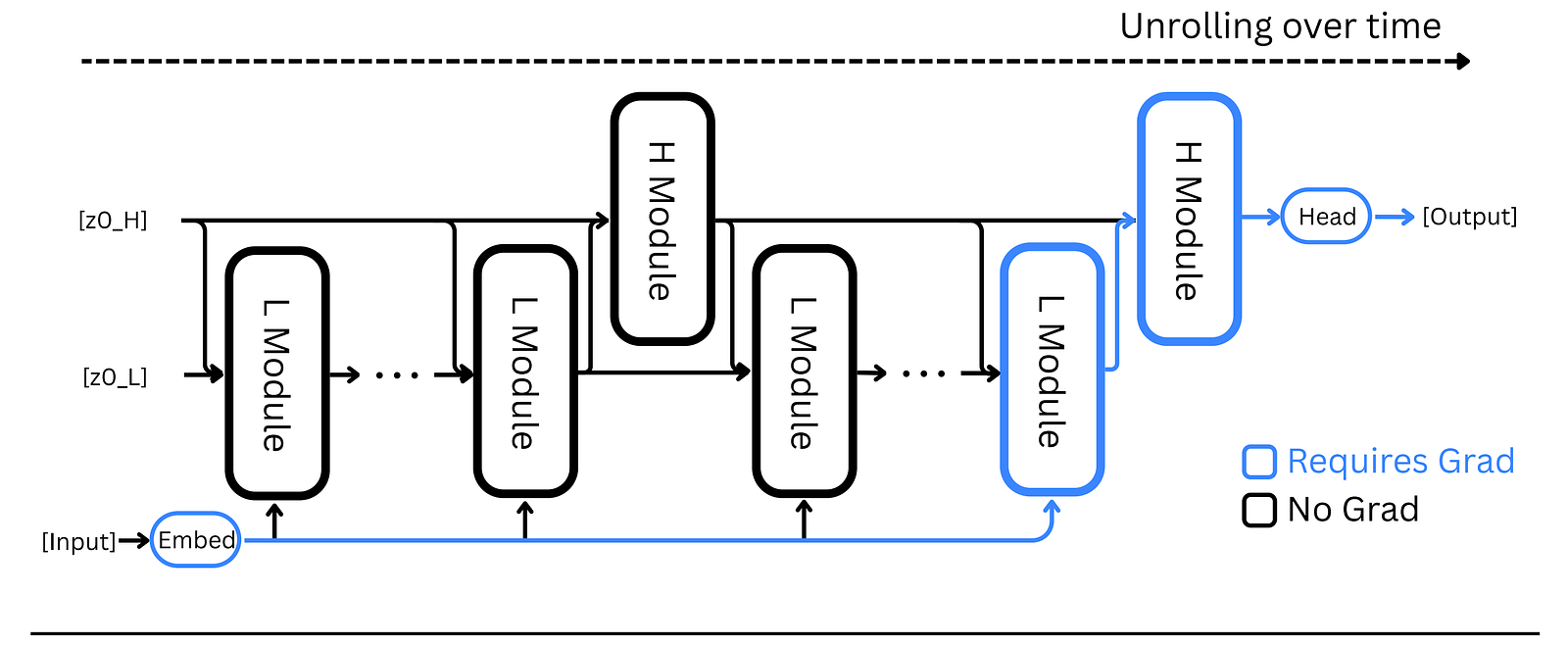
HRM solves this with One-Step Gradient Approximation.

With this approach, once a recurrent network converges to a fixed point, we can bypass unrolling through time and apply backpropagation in a single step at that final equilibrium point, treating all other intermediate states as constants.

The gradient flow goes like this:

Output head → Final state of the H-module → Final state of the L-module → Input embedding

This reduces the space complexity to O(1) memory (instead of previously O(T) memory).

HRM using One-Step Gradient Approximation

This method of One-Step Gradient Approximation is based on Deep Equilibrium Models (DEQ), which use the Implicit Function Theorem (IFT) to bypass Backpropagation through time.

Let’s understand the gradient computation step by step.

Consider a cycle k, at the end of which the L-module converges to a local equilibrium denoted by z*(L).

Given the current H-module state of z(k-1)(H), this step can be expressed as:

Based on this converged state of the L-module, the H-module performs a single update as follows:

Using a function F, this equation can be written more compactly as follows, where θ = (θ(I), θ(L), θ(H)):

The convergence point of the H-module z*(H) can be written in this form as:

Using the Implicit Function Theorem (IFT), the gradient of this point is:

Calculating the inverse of the Jacobian matrix in this equation is computationally expensive.

Therefore, it is approximated using the first-order term of the Neumann series as follows:

This simplifies the gradient to:

Using the Chain rule for θ(H), θ(L), and θ(I) i.e., the parameters of H-module, L-module, and the input network, respectively, the gradients are as follows:

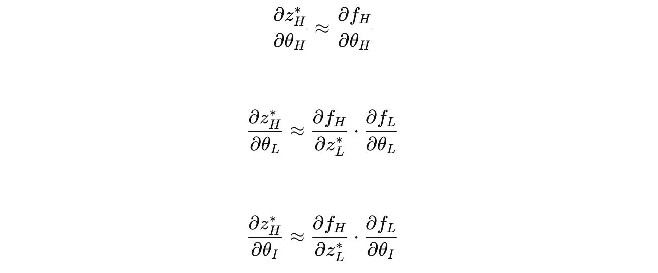
These are the one-step gradients used when training an HRM, which avoid storing complete state histories and backpropagating through time.

Training HRM Using Deep Supervision

Now that we understand the forward pass and the one-step gradient calculation process, let’s next learn how an HRM is trained overall.

For a data sample denoted by (x, y), where x is the input and y is the label, respectively, multiple forward passes are run.

Each of these forward passes is called a Segment.

The hidden states of the H-module and L-module after each segment (total segments are M, each indexed by m) are denoted by z(m) as shown below:

Given the state z(m — 1) from the previous segment, the next hidden state z(m) and its associated output ŷ(m) are calculated as:

The loss for the current segment is calculated as:

This is followed by a gradient update as follows:

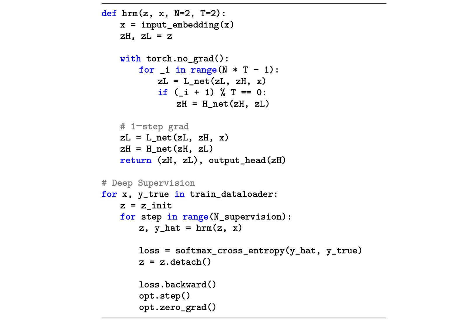
One of the critical aspects of this training method is that the hidden state from a segment is detached from the computation graph before it’s used in the next segment.

This means that gradients from later segments don’t flow backward into earlier ones.

As a result, the model uses a simple, one-step gradient estimate instead of full backpropagation through time.

The pseudo-code of this technique, called Deep Supervision training, is shown below.

Pseudocode of Deep supervision training of an HRM written in PyTorch

Thinking Fast & Slow With Adaptive Computational Time

Remember that we talked about a halting mechanism when we learned about the overview of HRM?

Let’s discuss it in detail next.

The human brain functions in two modes of thinking and dynamically modulates how long each mode runs for, given the task complexity and the potential reward one might get from completing the task.

These two modes are:

Fast and automatic thinking (“System 1”)
Slow and deliberate reasoning (“System 2”)

Borrowing from this insight, researchers add an adaptive halting strategy to HRM, which decides how many forward passes (segments) it must train for.

After the end of each segment, Q-head, a learned function, takes the final hidden state of the H-module and predicts two Q-values (represented by Q̂(m)):

These Q-value estimates the value of either halting or continuing computation after a segment.

The Q-head function is as follows, where σ is the sigmoid function, θ(Q) represents the Q-head parameters, and z(m)(H)(NT) is the H-module’s state after segment m (N x T timesteps):

The halt or continue action is chosen based on a randomized strategy, which goes as follows.

Given that M(max) and M(min) are the maximum and minimum number of segments, respectively, the value of M(min) is:

determined by sampling uniformly with probability ε from the set {2, … , M(max)} (which encourages the model to think longer during training with probability ε)
set to 1 with a probability 1 - ε (which allows early halting)

After segment m, the model halts if either of the following conditions is met:

If M(max) or maximum segments are reached

If at least M(min) is reached, and if the predicted Q-value of halting exceeds that of continuing

The Q-head that decides whether to halt or continue computation is trained using Q-learning in the form of an episodic Markov Decision Process (MDP).

The state of the MDP at segment m is given by z(m), and the action space is {continue, halt}.

Choosing continue yields a reward of 0 and the state transitions to z(m + 1).

Otherwise, choosing halt ends the episode and returns a binary reward based on prediction correctness (Reward is 1 if the prediction is correct, otherwise 0.)

The Q-learning targets, as shown below, are the expected reward for taking each action at segment m, and they are used to train the Q-head of the model.

The target value for the halt action is a binary reward where the reward is 1 if the prediction is correct, otherwise 0.

The target value for the continue action is estimated as follows:

Based on this, the total loss for training an HRM is given by:

where the first loss term is for better task-solving (increases accuracy), and the second loss term is for training the halting policy.

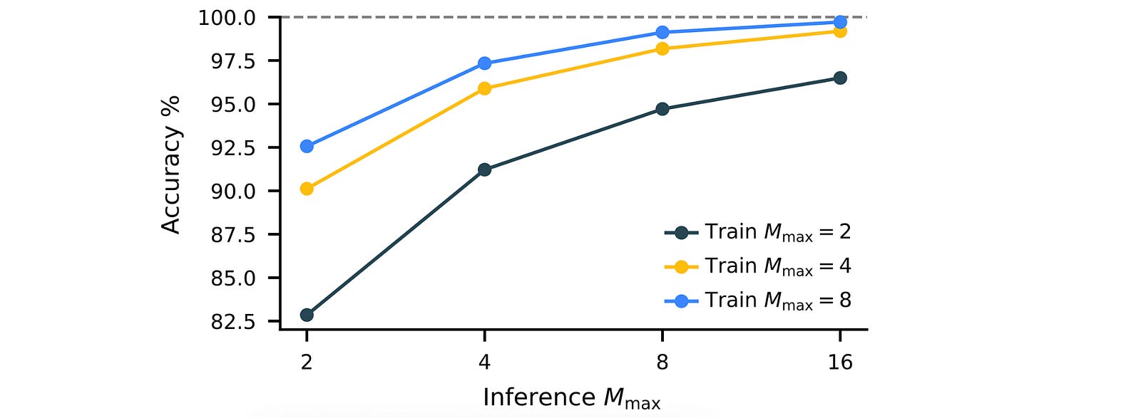
Thanks to this approach, HRM can scale well on hard tasks at inference time by simply increasing M(max) (a fixed hyperparameter) without any further architectural modifications.

HRM trained with a specific M(max) improves its accuracy on the difficult Sudoku solving task when M(max) is increased at inference.

Diving Deep Into The Architectural Details Of An HRM

Now that we know the specialized techniques that make an HRM work, let’s learn about its architecture next.

An HRM is a sequence-to-sequence model with hierarchical, transformer-based recurrent reasoning modules.

(The term “recurrent” means that the same Transformer module is looped over multiple reasoning steps, each time refining its hidden state before producing the final output.)

Its input and output are represented by token sequences x = (x(1), ... , x(l)) and y = (y(1), ... , y(l′)) respectively.

The input tokens are mapped to a vector representation using an embedding layer f(I).

An output head f(O) converts its final hidden state z into token probability distributions ŷ using the softmax function.

The token-level sequence loss used is as follows:

Token-level sequence loss where p(y(i)) is the predicted probability that the distribution `ŷ(i)` assigns to the token y(i)

Both H-module and L-module are implemented as an Encoder-only Transformer with similar architectures and dimensions.

All Transformer components use:

Rotary Positional Encoding (RoPE) for better position handling
Gated Linear Units (GLU) in place of standard feedforward layers
RMSNorm (without scale/bias parameters)
No bias terms in linear layers to simplify and stabilize training

A Post-Norm architecture (normalization after each residual block) is used, and all parameters are optimized using the Adam-atan2 optimizer.

A Glimpse Into The Spectacular Performance Of HRMs

That was a lot of theory to learn about! Let’s learn about what happens when an HRM is put to the test.

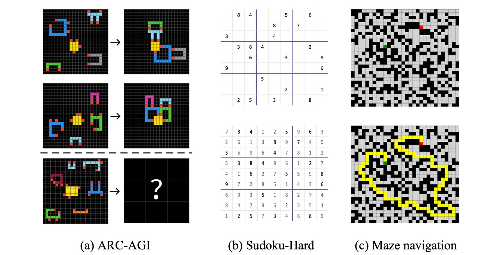
HRM is tested on three tough benchmarks:

ARC-AGI Challenge: A dataset of questions that test general intelligence using IQ-style puzzles that require inductive reasoning.
Sudoku-Extreme: A dataset of highly challenging 9 × 9 Sudoku puzzles
Maze-Hard: A dataset of complex 30 × 30 mazes that tests optimal path finding capability

Visualisation of the tasks in the three benchmarks

For each benchmark task, the model is initialized using random weights and trained using a small dataset of around 1000 input-output pairs.

(This is considered a small number because conventional reasoning LLMs are trained on hundreds of thousands/ millions of examples.)

Reiterating this fact, an HRM is trained from scratch, directly on the input–output pairs for the target tasks. No pretraining or training on Chain-of-Thought (CoT) labels occurs during its training.

Next, to the results!

Results show that HRM outperforms all baselines on ARC-AGI-1 and 2 benchmarks.

The same goes for Sudoku-Extreme and Maze-Hard benchmarks, where an HRM again beats all baselines.

With just 1000 training samples, while other baselines have 0% accuracy on these tasks, the HRM achieves an accuracy of 55% and 74.5% on Sudoku-Extreme and Maze-Hard, respectively.

Performance comparison between HRM and other baselines. “Direct pred” baseline refers to *direct prediction without CoT and pre-training*, using the exact training setup of HRM but replacing its hierarchical architecture with a standard Transformer.

What Does An HRM Do Internally To Perform This Well?

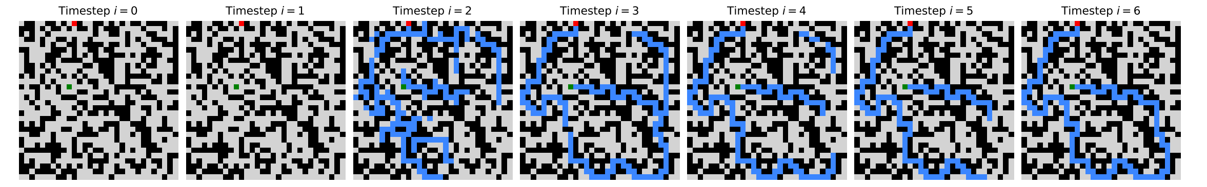
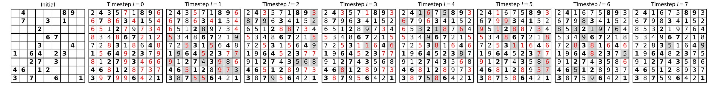
To understand the internal algorithms an HRM uses to achieve such impressive results, researchers try to visualize its intermediate states.

At each timestep, they perform a forward pass through the H-module.

*The intermediate state of the H-module at timestep i, computed using the current hidden states of both the H-module and L-module, given the H-module’s parameters θ(H)*

The output is then decoded (ȳ(i)) and visualised as shown in the image below.

The intermediate prediction at timestep i, obtained by decoding the intermediate H-module state z̄(i) using the output function f(O) with parameters θ(O).

It is seen that in the Maze-Hard optimal path finding tasks, the HRM explores multiple potential paths in parallel, gradually discarding the suboptimal paths and building a rough solution which it refines over multiple iterations.

Visualization of intermediate predictions by HRM on a Maze-hard benchmark task, where blue cells indicate the predicted path

When solving tasks from Sudoku-Extreme, a strategy similar to Depth-first search is used, where the HRM explores potential solutions and backtracks if it encounters dead ends.

Visualization of intermediate predictions by HRM on a Sudoku-Extreme benchmark task, where red cells show incorrect answers, and grey indicates changes from the previous timestep

When solving the ARC-AGI tasks, a strategy similar to Hill-climbing optimization is used, where the HRM gradually applies small, step-by-step modifications to refine its output until a solution is reached.

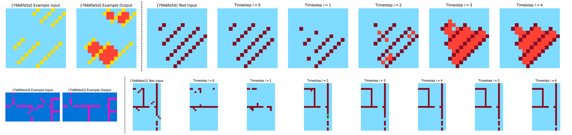
Visualization of intermediate predictions by HRM on a ARC-AGI-2 task

While it’s difficult to tell exactly how an HRM works internally, these visualizations still give us insight into how it is highly adaptable to different tasks and uses different reasoning strategies for each one of them.

HRMs are also Turing-complete, or computationally universal, when given sufficient memory and time constraints.

The brain-inspired HRM architecture is very impressive, given that it solves such difficult tasks that all other state-of-the-art reasoning LLMs fail on with just 27 million parameters and training on only around a thousand examples.

While we are still far from fully replicating the human brain, which performs so well in general-purpose tasks using little energy compared to LLMs of today, research like this represents a meaningful step toward that goal.

Source Of Images

All images used in the article are created by the author or obtained from the original research paper unless stated otherwise.

Subscribe to ‘Into AI’ — a newsletter where I help you explore the best and latest in Artificial Intelligence from the ground up by dissecting the original research papers.

Into AI

Discussion about this post

Ready for more?