How RNNs Work (And Why Everyone Stopped Using Them)

A gentle walkthrough of how Recurrent Neural Networks (RNNs) work, and the math that breaks them.

Dr. Ashish Bamania and Jose Parreño Garcia

Feb 07, 2026

Reshape (Affiliate Partner)

Tired of trying to reach your weight loss goals and failing each time? We have all been there. But not anymore.

It’s time to start seeing real results with Reshape!

Just snap a photo or say what you ate, and instantly get precise calorie, macro, and nutrient tracking with Reshape’s AI, skipping all that tedious logging work.
Get workout plans tailored for your equipment, schedule, and fitness level that change as you progress. Whether you’re building muscle, losing fat, or getting stronger, these plans adapt to your needs.
Your 24/7 AI coach, Fio, is a personal trainer in your pocket that provides instant feedback on your form, meal ideas, and motivation whenever you need it.
Track everything that matters in one powerful dashboard: meals, workouts, sleep, steps, and body composition, with easy Apple Health integration.
Track your weekly insights to learn what’s working for you so that you keep winning each and every day.

Use the code “INTOAI” for a free Reshape Pro trial and join 45K+ people who have transformed their bodies with Reshape. Your smarter fitness journey starts now!

Try Reshape for FREE!

This week’s newsletter is written by Jose Parreño Garcia. He is a senior Data Science manager at Skyscanner.

He regularly shares insights on building effective teams, developing leadership skills, and advancing careers in Data Science and Machine Learning through his newsletter, Senior Data Science Lead.

You can also find him and stay up to date with his content on LinkedIn.

This week, I went all the way back to 2017. That’s when the now-legendary ‘Attention is All You Need’ paper came out — the one that introduced the world to Transformers, and set the foundation for everything from ChatGPT to image generation to code-writing copilots.

And sure, I could jump straight into explaining how Transformers work. But given the impact these models have had — and the fact that you probably see the word “attention” 30 times a week now — I thought it would be worth taking a step back (actually 2 steps back).

Before we can truly understand Transformers, we need to understand where they came from. And that means revisiting the architectures that paved the way: Recurrent Neural Networks (RNNs) and Long Short-Term Memory (LSTM) networks.

In this blog post, I am diving into RNNs.

We will walk through what they are, how they work, and most importantly, why they struggle. By the end, RNNs will feel like a clever little for-loop with memory instead of scary maths magic.

Ready? Let’s jump in!

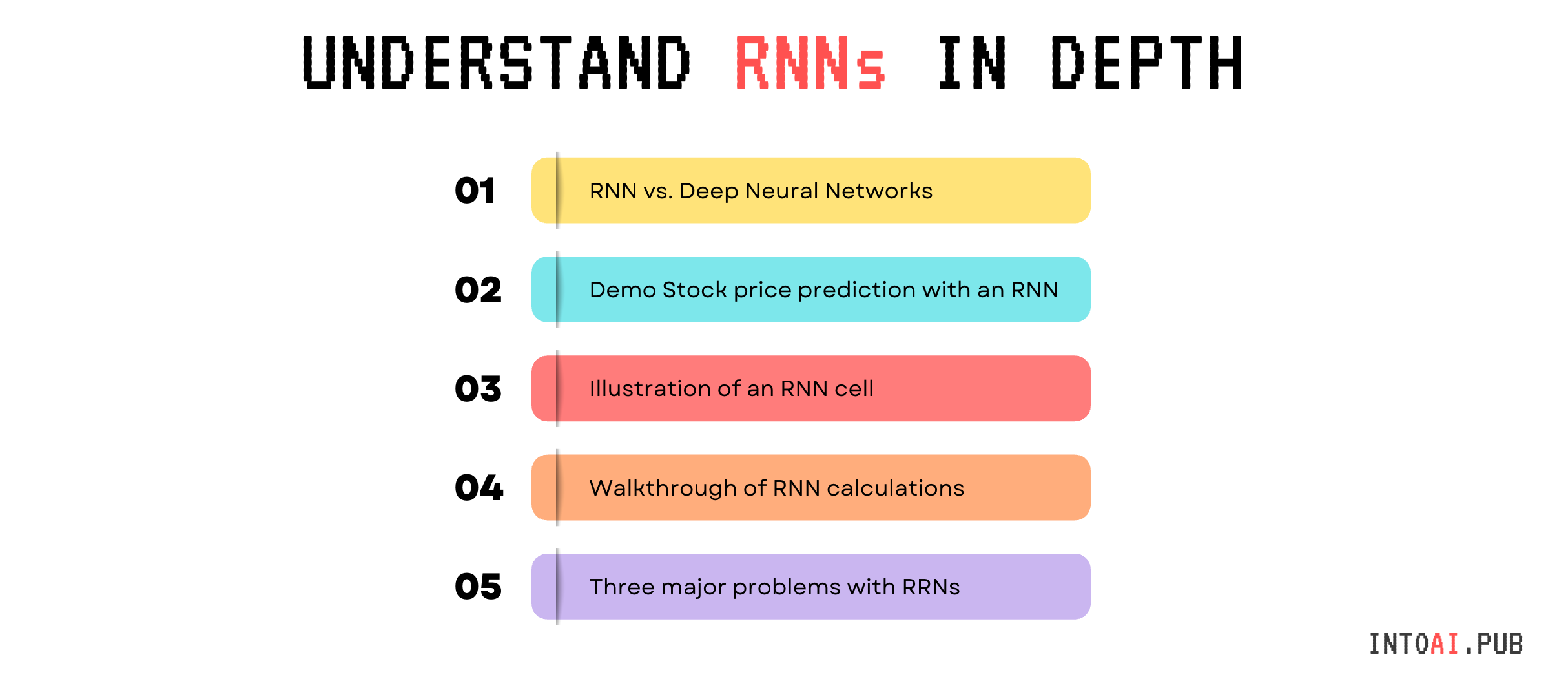
What we will cover in this article

How is an RNN different from a classical Deep Neural Network? (or other classical sequence models)
Introducing a made-up use case with 3 data points for Stock price prediction
The scary official diagram of an RNN cell. (Don’t worry, we will break it down super easily.)
A walkthrough of RNN calculations (And you will see how the maths is not that scary after all.)
Three problems associated with RNNs

How is an RNN different from a classical Deep Neural Network?

I assume in this post that you have worked with (or are familiar with) the basics of classical Deep Neural Networks (from here on, DNNs).

If my assumption is correct, then the diagram below should feel really familiar. It is a diagram of a DNN with:

X: A set of input nodes, representing the variables you want to use for prediction.
H1, H2: 2 hidden layers with 4 nodes. This is where the parameters that learn how to dial up or down specific signals from X. Basically, the knobs the model adjusts to learn.
Y: The prediction node. In this case, it’s only 1 for simplicity.

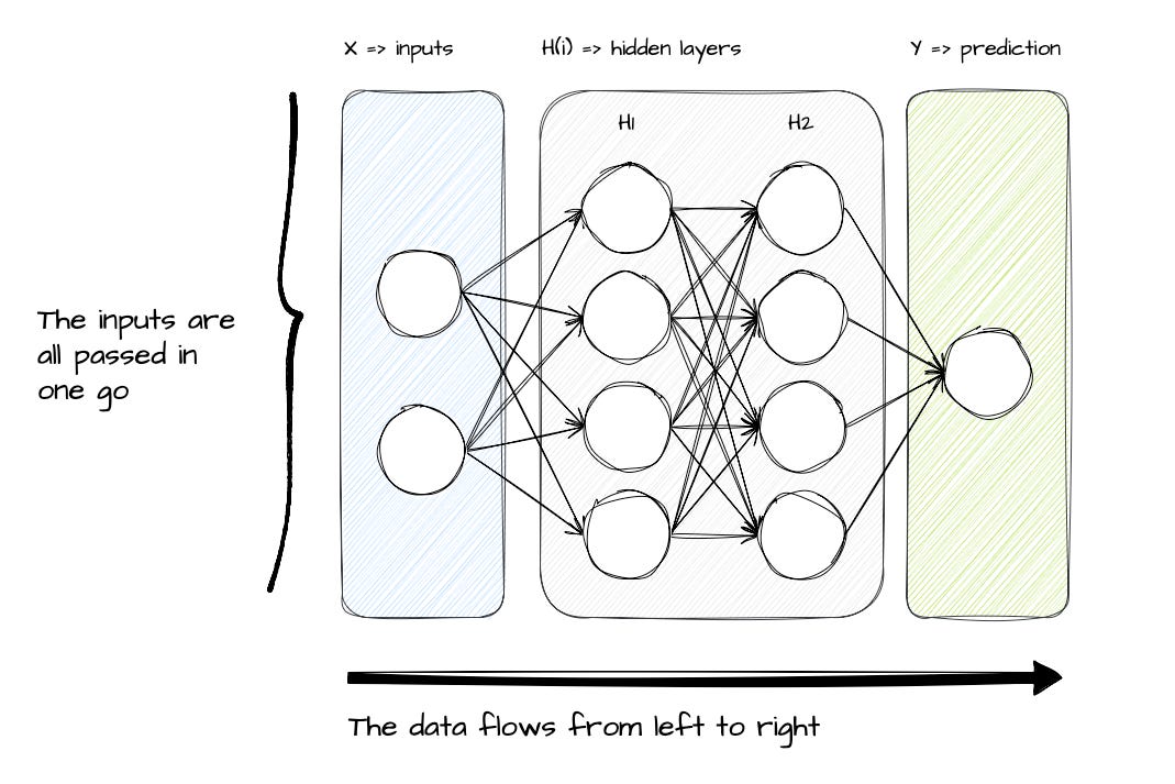
Diagram of a classical Deep neural network (DNN)

Now, there are 2 main things to highlight in this diagram:

The DNN processes all the data at once.
You see the X input? From a DNN’s perspective, it’s a torrent of data, all pushed and processed at once. There is nowhere in this diagram that the network can say, “Hey, can you just send me X1 and X2 first, and then I can process X3 and X4?”.
The DNN is feed-forward (or sequential).
In other words, the data flows from left to right (from X → Y). There is nowhere in this diagram that a node can stop the data flow and ask: “Hey, what data did I have in the previous step?” It is oblivious to that.

DNNs are really powerful, but they are also “memory-less”

DNNs are “memory-less” because of the two points mentioned above. And being “memory-less” means that DNNs really struggle to predict when sequence or order matters.

Take a simple stock price prediction scenario. The only way that DNNs can consider what happened yesterday or the day before is if you tell them what matters. This is usually done by manually creating features like:

Yesterday’s price
A moving average over the past 7 days
A sine-transformed day-of-week feature to capture seasonality

But wasn’t Deep learning supposed to eliminate Feature engineering?

Yes (and no).

Neural networks do learn internal representations (i.e., “features”) from raw data. But when it comes to sequences, classical deep neural nets still need all the help they can get (so, kind of back again to square one, where we have to feature engineer stuff…)

This is where Recurrent Neural Networks (RNNs) come in.

Recurrent neural networks (RNNs) are a class of artificial neural networks designed for processing sequential data, such as text, speech, and time series, where the order of elements is important.

Their two main characteristics are:

RNNs process one input at a time.
Instead of taking all of the input X in one big gulp, RNNs look at one data point at a time — like reading a sentence word by word, or stepping through a stock price day by day. This allows them to focus on how each input evolves over time.
RNNs are recursive.
Yes, the information flows left to right, but at each step, it can also look at what happened before (kind of a right-to-left motion). It’s like a left-to-right with memory.

Don’t worry if this feels dense right now, we will break it down step by step.

By the end of this post, you will not only understand what “recurrent connections” mean, but you will also see why RNNs became a foundational architecture for handling sequences.

Introducing a made-up use case for Stock price prediction

Ok, before we get into the RNN section, let me introduce you to the simplest stock price prediction exercise in the course of human history.

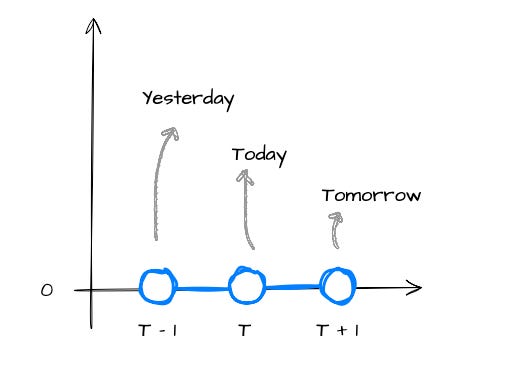
The diagram below shows a toy time series where:

For simplicity, all stock prices are set to 0.
We have 3 data points.
The idea is to use yesterday’s and today’s stock prices to predict tomorrow’s stock price.

I want to introduce this in such a simple way because:

I want to actually show you the maths of the RNN using super simple numbers.
Labelling each step as yesterday, today, and tomorrow will help anchor the RNN diagrams that follow.

Let’s keep this mental model in our back pocket — it’s going to make the scary-looking RNN diagrams feel a lot less scary.

Ok, now we are ready to get scared by a diagram of an RNN cell!

The scary official diagram of an RNN cell

So far, we have discussed how RNNs differ from classical DNNs because they remember their past. But what does that actually look like inside the model?

Well... time to face the infamous RNN diagram.

It might look like a tangle of wires and equations at first, but don’t worry, we will walk through it slowly, tie it back to the stock price example, and by the end, you will see it’s just a simple process of multiplication, addition, and a squiggly activation function or two.

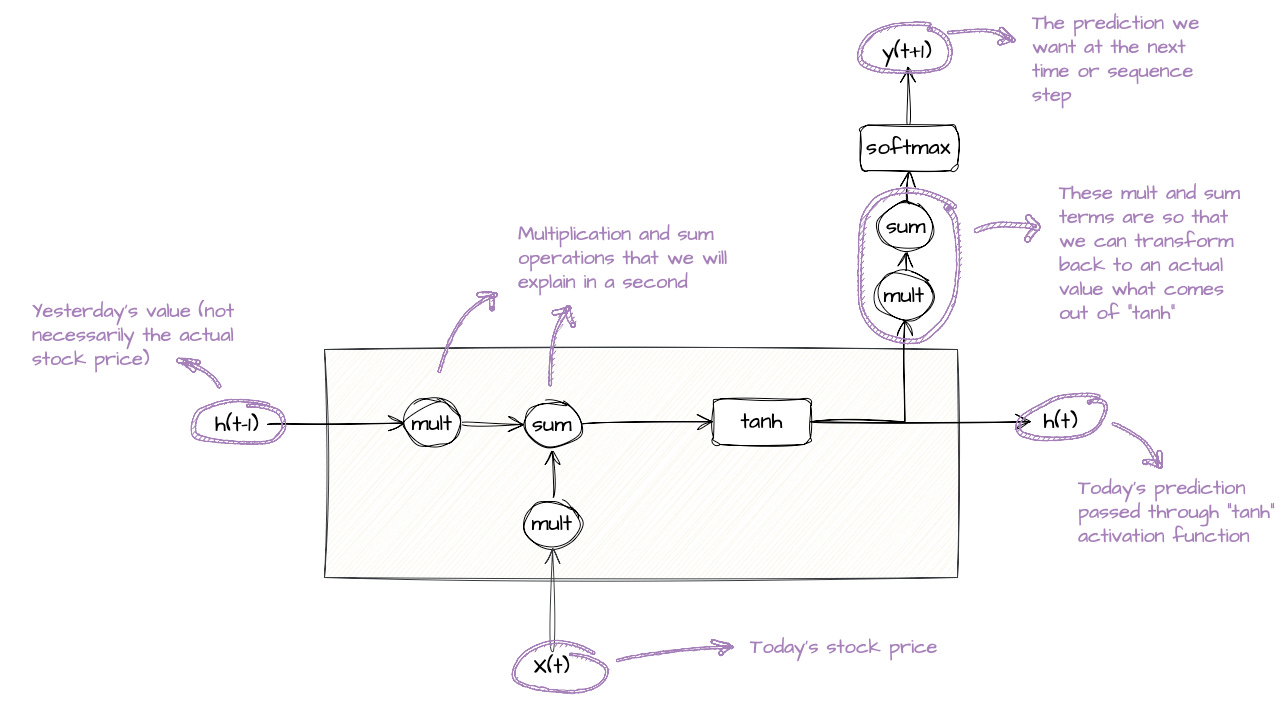
The diagram below is a vanilla RNN cell.

I can sense you sweating… a flow diagram? With parameters? With maths operations? Ok, let’s break it up so that you don’t have to process it all at once.

Here are the elements to focus on:

Note the X, h and Y elements (similar to the classical DNN diagram).
X(t) represents today's data point, h(t-1) is what came from yesterday, h(t) is what is passed to predict tomorrow, and Y(t+1) is the predicted data point.
Y(t+1) represents the prediction that we want.
tanh and softmax are just activation functions. The same kind you have seen in regular neural networks, so nothing special for RNNs. They take raw values and squash them into a friendlier range, like between -1 and 1 (for tanh) or 0 and 1 (for softmax).
Finally, there are a couple of blobs with mult and sum. These are just visual aids so that you can see the operations in action when we pull the numbers in.
There are maths operations outside of the cell. These are basically there just so that we can transform a squashed value coming out of tanh, into a real value that makes sense. For example, transform 0.9 coming out of the tanh function to maybe $5.

✍️ Quick note

Technically, the RNN makes a prediction y(t) after seeing input x(t) and memory h(t-1).

But since in our toy example we are trying to predict the next value, it’s tempting to call it y(t+1) — just know that it’s really y(t) in the math, but the target we are aiming for is the value at t+1.
I purposely named it y(t+1) for pedagogical reasons for this post.

Let’s map this diagram with the theoretical RNN math function

In the image below, I have added the math functions that lead to the two outputs from the RNN cell: y(t+1) and h(t).

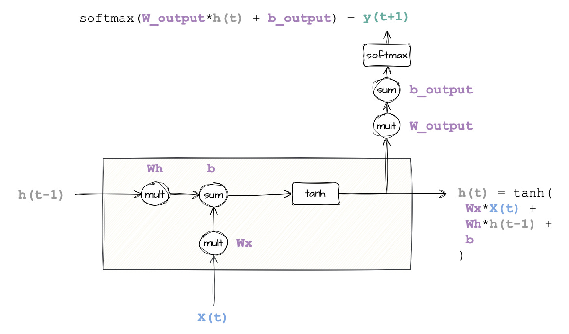
So, if we wanted to either predict an output (Y) or carry to the next stage (h), then the neural network should learn:

Wx: This is the weight applied to today’s data, X(t). It controls how much the model should care about today’s stock price. Extreme case, if Wx = 0, then this means we don’t care about X(t) because Wx * X(t) would yield 0.
Wh: This is the weight applied to the previous hidden state, h(t–1). It tells the model how much to rely on memory. If Wh = 0, the past is forgotten.
⚠️ Don’t misinterpret h(t-1) by thinking it is yesterday’s stock price. It is what comes out of the cell (with its multiplications, sums, and activation functions) applied to yesterday’s stock price.
b: This is the bias term. Think of it as a small correction applied regardless of the input. It’s important in training, but not very interesting for understanding how RNNs work conceptually (as it affects DNNs the same way). If you want to deep dive, check this link.

I believe that only when we plug in numbers to these diagrams will we start really understanding what is happening inside the RNN. Let’s do this next.

A Walkthrough With Real Numbers

Alright, time to take what we have learnt and run it step by step. Instead of just showing the internals of a single RNN cell, we’ll now “unroll” it (you will see what that is in a second).

This will finally answer the big question: how does an RNN actually use the past to predict the future?

How do we represent tomorrow’s prediction diagrammatically?

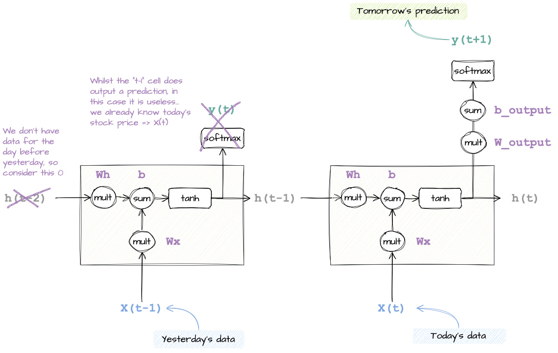
Pretty simple. We just copy and paste the same RNN cell forward in time, one per data point in our sequence.

In our toy stock price example, we only have two data points (t–1 and t), so we unroll the cell twice in order to make a prediction at t+1.

And this is why they are called recurrent, because the same logic is applied over and over, like a for loop.

Cool, now that you are comfortable with what happens inside a single RNN cell, let’s walk through this unrolled diagram in detail to ensure we are all on the same page.

We begin by plugging in yesterday’s stock price. Because there is no data prior to yesterday, we can ignore the previous hidden state input h(t-2).
Using both math functions, we then calculate y(t) and h(t-1). From these two, only h(t-1) is useful for us. This is the value that describes the memory, and that will be passed to the next cell. y(t) is irrelevant, so we ignore it.
Finally, we plug in today’s data and run through the relevant maths operations to calculate y(t+1). You can see from the diagram that the RNN is using today’s data X(t) and yesterday’s data h(t-1) from memory to calculate what could happen tomorrow.

💡 An important highlight: Shared weights and biases

“Wait a sec... you are using the same Wx, Wh, and b in both cells. Shouldn’t they be different?”

Great question! This is the part that makes RNNs elegant, but also tricky (you will see at the end how these shared weights break an RNN’s learning process).

Unlike feedforward layers that might learn new weights for every input, an RNN cell reuses the same weights at every timestep. That’s the “recurrent” part. An RNN not only repeats the cell structure, but it also repeats the exact same function with the same learned parameters.

So yes — Wx, Wh, and b are constant across time. What changes is the input x(t) and the memory from the previous step h(t–1), which is how the model updates its thinking as it moves forward.

Plugging numbers into the diagram

Before doing some basic maths, let’s talk about the numbers being used:

Note how I substituted Wh, Wx, b, W_output and b_output with numbers. I made these numbers up, but they are the ones the neural network would tweak during its learning process.
The input data points are the ones we know from the time series. X(t-1) and X(t) are both 0.

Now we are ready to take pen and paper and perform all the calculations in this diagram.

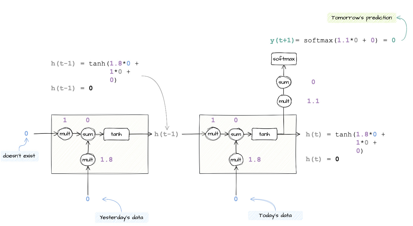
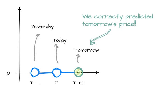
Plugging in all the numbers, y(t+1) comes out to be 0. Nice, this is what we expected from our mock stock price time series!

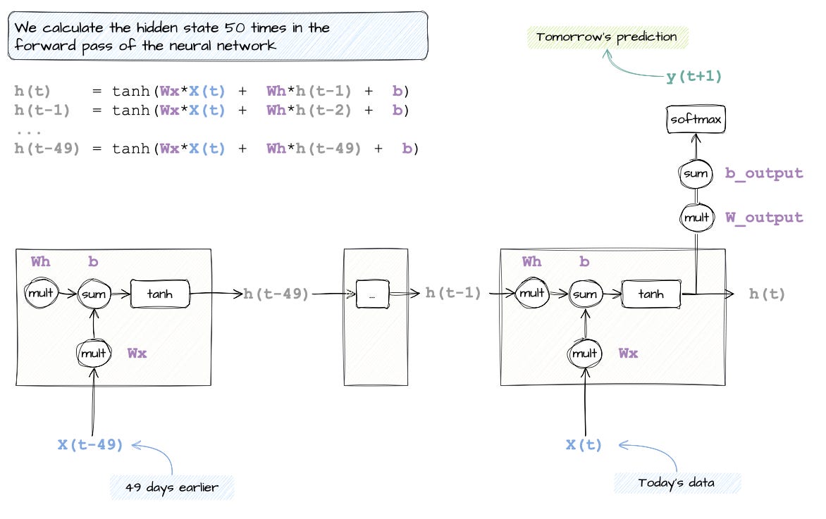
What would the diagram look like if we had 50 data points?

Well... you would copy the RNN cell forward 49 times, just like a for loop with 50 iterations (luckily for me, I am not drawing that diagram...)

But structurally, nothing changes. You still:

Reuse the same weights
Pass memory from each time step to the next
And only apply the final output prediction where it matters, which is usually the last cell in the sequence

What we learn from the above examples is that:

RNNs reuse the same weights and biases at each step.
Hidden states h(t) are like memory, passed forward through time.
Outputs y(t) are generated by applying a linear transformation and softmax on the hidden state.
Even a dumb toy dataset of all zeros reveals the internal mechanics beautifully.

That wasn’t that hard, right? Well, I have bad news for you…

Three Major Problems With RNNs

These vanilla RNNs are never used for real-world use cases because they come with three big problems:

They are slow to train.
They suffer from the problem of vanishing gradients
They suffer from the problem of the exploding gradients

Let’s cover these in detail in their own sections.

Problem 1: Training a vanilla RNN is very slow

Deep Neural Networks (DNNs) process all their inputs at once in a single forward pass. Everything flows from left to right, layer by layer. That means training can occur in parallel across many data points and GPU cores.

This is not the case with RNNs.

Because RNNs depend on previous hidden states, they are inherently sequential. You can’t calculate h(t) until you have calculated h(t–1).

It’s like reading a book: you can’t understand chapter 5 until you have read chapter 4.

RNNs make you walk through time, one step at a time, and this sequential dependency kills parallelism.

That is the first problem: RNNs are powerful, but they pay for it in training speed.

Problem 2: The problem of the Vanishing gradients

To explain this problem, I would have to take some mathematical shortcuts. To really know what is happening under the hood, you need to be familiar with the chain rule used in backpropagation. But showing the full impact of vanishing gradients using the backpropagation formula would be overkill.

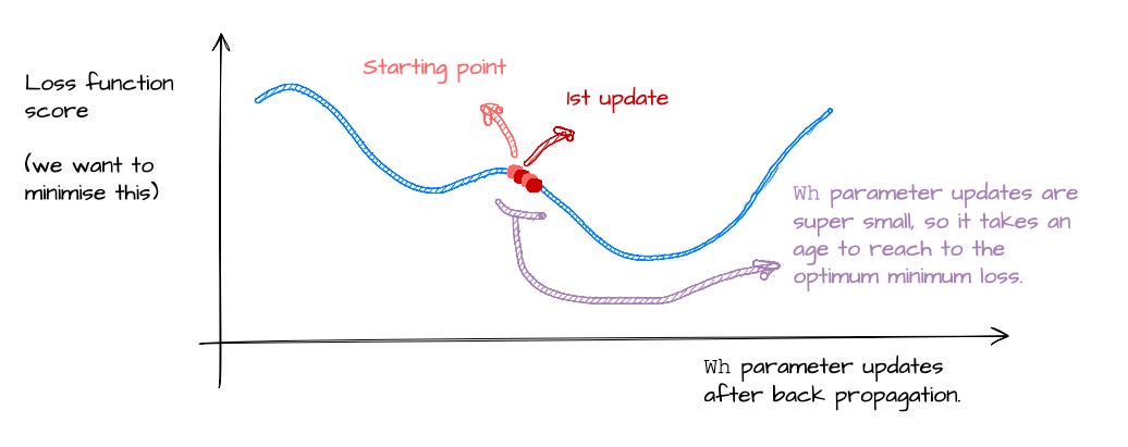
Let’s zoom in on just one parameter in the RNN, i.e. Wh, the weight that is multiplied by the previous hidden state.

In our earlier 3-step example, Wh was used once (just one multiplication). But, if you are training an RNN for 50 timesteps (say, 50 days of stock data), that means Wh shows up 49 times in the full chain of calculations.

When the model tries to update Wh via backpropagation, mathematically, the gradient is multiplying Wh over and over again, kind of like:

Uh-oh. What happens when Wh < 1?

Try plugging in Wh = 0.5:

That’s basically zero. This means that the update to Wh during training is so tiny, it’s like the model is frozen. It can’t escape its starting point. It just sits there, unable to learn anything useful.

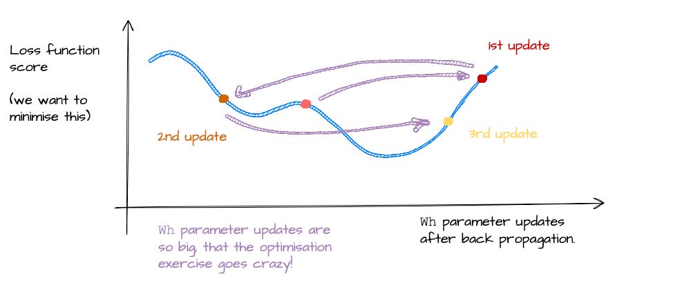
Problem 3: The problem of the Exploding gradients

This is the opposite problem. If vanishing gradients are the slow death of learning, exploding gradients are the chaotic opposite.

What happens when Wh > 1? Say Wh = 1.5.

That’s nearly a billion. This means that during backpropagation, the gradient becomes massive. And with a gradient that large, your weight update becomes a wild jump.

The result is that your model overshoots the loss minimum, bounces around the optimisation landscape like a drunk pinball (love that game), and probably never converges.

This is the exploding gradients problem. Same root cause as vanishing gradients — compounding multiplications through time — but now the problem is too much signal, instead of too little.

What’s next: How LSTMs fixed all of this (mostly)

With everything we have covered, you might think, “Hey, that vanilla RNN was easy enough to understand, but with the stated problems, it also looks pretty useless, right?”

I would mostly agree. Training a vanilla RNN is not impossible, but it requires skill, feature engineering, fine-tuning, and time. The vanishing and exploding gradient problem is the one that mostly holds back an RNN.

This is why LSTMs were introduced.

LSTMs are improved versions of RNNs. With built-in mechanisms (called Gates) to decide what to keep, what to forget, and what to pass forward, they were designed specifically to beat vanishing and exploding gradients at their own game.

LSTMs are for the next post, where we will explore how they work and why they became the go-to tool for sequence modelling… at least until Transformers came along.

Now, I want to hear from you!

In this post, we broke down how RNNs work, from the vanilla cell structure to why they struggle to train in the real world.

We kept it simple, even used an all-zero dataset, and uncovered the quiet math that makes RNNs nearly impossible to scale.

But now I’m curious about your experience.

Have you ever built or trained an RNN model?
Did you run into vanishing gradients or the joys of exploding updates?
Maybe you were introduced to LSTMs (or GRUs) straight away and skipped vanilla RNNs altogether?
Or maybe you are just now connecting the dots between hidden states, time steps, and why Transformers were such a leap.

Drop your thoughts, experiences, or lingering questions in the comments. I would love to hear how you’ve approached sequence modelling in your ML journey.

Thanks again to Jose Parreño Garcia for writing this week’s newsletter.

Don’t forget to subscribe to his newsletter and connect with him on LinkedIn.

This article is free to read, so share it with others. ❤️

If you want to get even more value from this publication and support me in creating these in-depth tutorials, consider becoming a paid subscriber.

You can also check out my books on Gumroad and connect with me on LinkedIn to stay in touch.

A guest post by

Jose Parreño Garcia

I write about Data Science, Machine Learning and leading data teams. I have built teams from scratch and lead 50+ data scientists @Skyscanner. Now, I share my experience with you.

Discussion about this post

Ready for more?