


✨ This newsletter features new research from Pathway. ✨
BDH-CQ is a 150M-parameter reasoning model that breaks the previously reported cost-accuracy Pareto frontier in ARC-AGI-1 and sets a new state-of-the-art for benchmark cost efficiency.
The model learns each new task from the examples it’s shown at inference time and progressively updates a recurrent memory to reason in latent space before giving an answer.
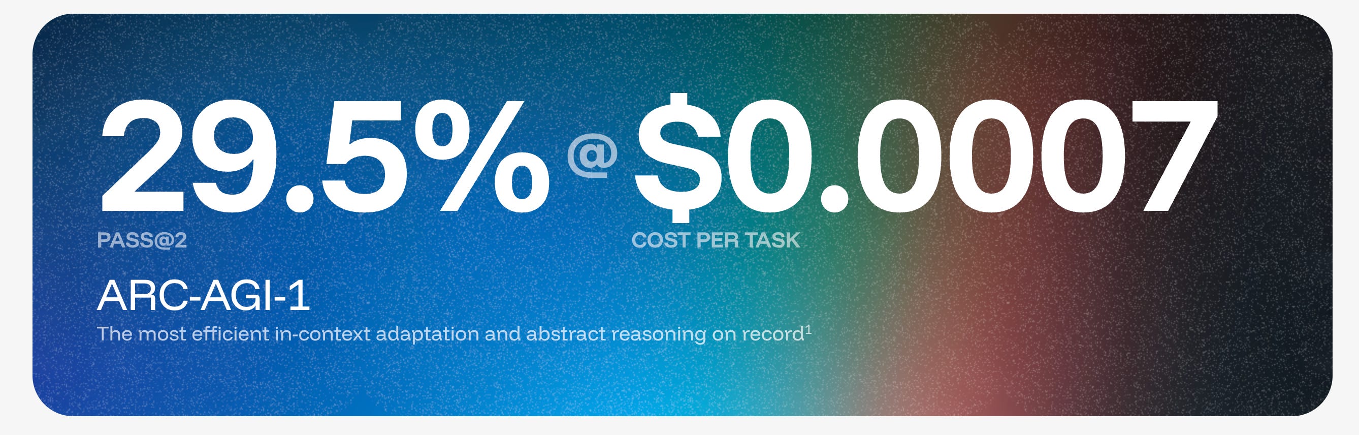
It achieves 29.5% pass@2 on ARC-AGI-1 at an inference cost of $0.0007 per task.
Although this is not the highest-accuracy result, BDH-CQ is ~57x cheaper than GPT 5.6 Luna (Low), which scores 34.2% (only 4.7% higher) at $0.040. Even after OpenAI announced a recent 80% reduction in API price, BDH-CQ is still ~11x cheaper than GPT 5.6 Luna (Low).
👨🏻💻 Read more about this research using these links: Hugging Face | ArXiv | Blog
Sponsor this newsletter to reach 12,000 smart AI engineers and leaders.
While requests can be processed one at a time as they arrive (sequential/ serialized processing), batching them is one of the best ways to improve LLM throughput. A scheduler decides how batches are formed and updated.
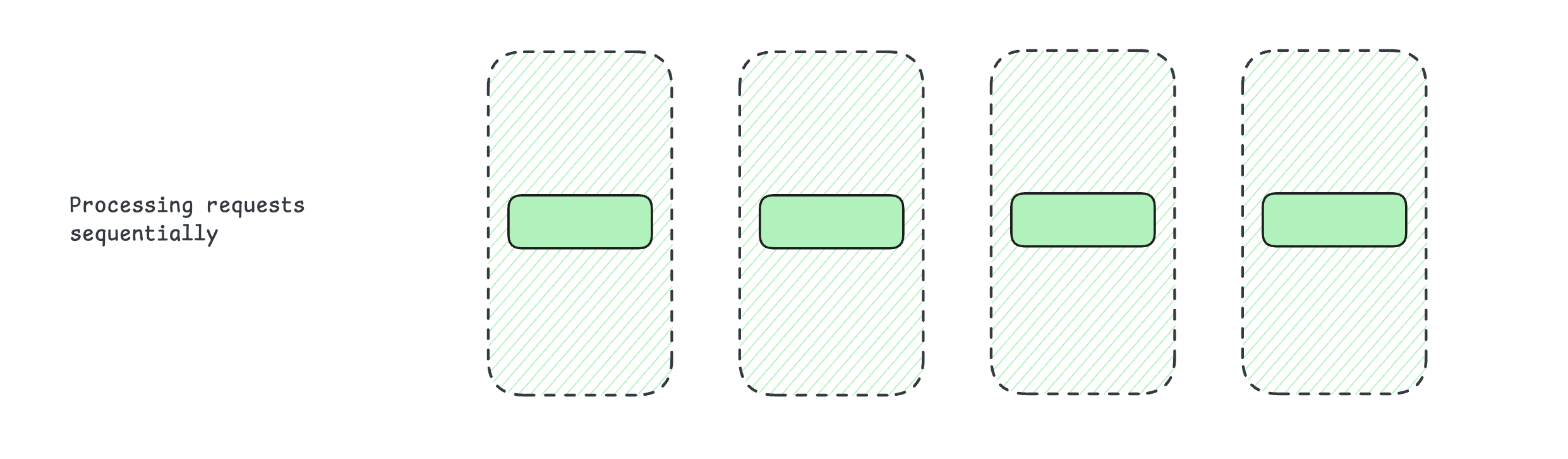
Here are the batching and serving strategies commonly used in modern inference architectures.
1. Static batching
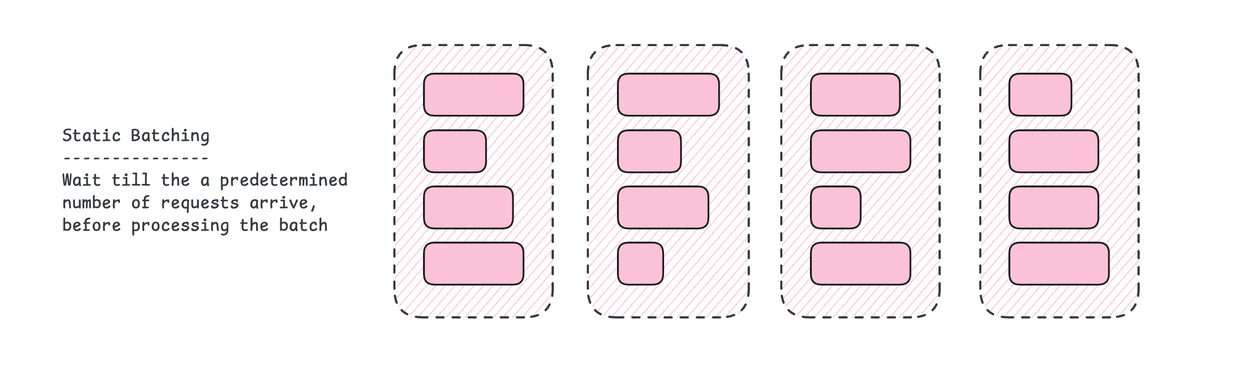
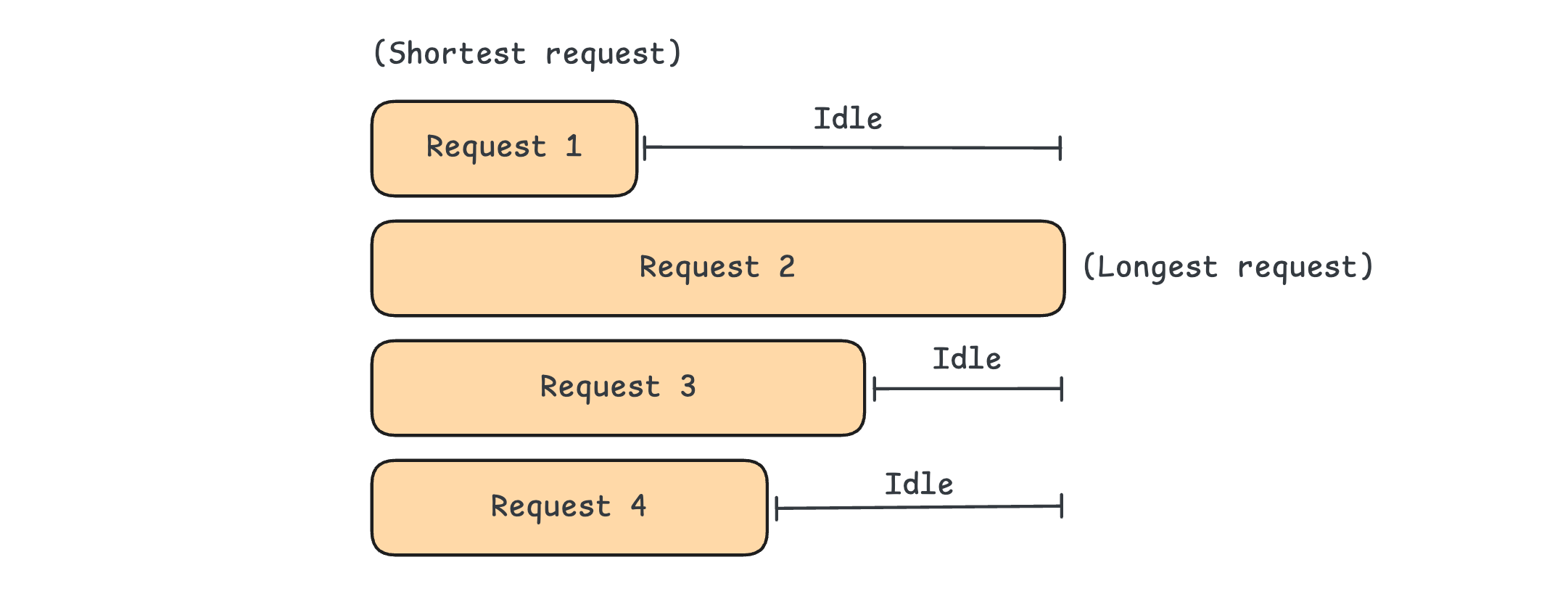
Static batching involves grouping incoming requests, and when a fixed preset number of requests (batch size) is reached, processing them together as a batch.
This is a simple batching strategy to implement, but it comes with high latency, as the preset batch size must be reached before processing requests begins. Also, the GPU has to wait for the longest request to finish before returning the batch outputs.
This strategy is used mainly for offline batch jobs or online inference systems with low, predictable traffic.
2. Dynamic batching
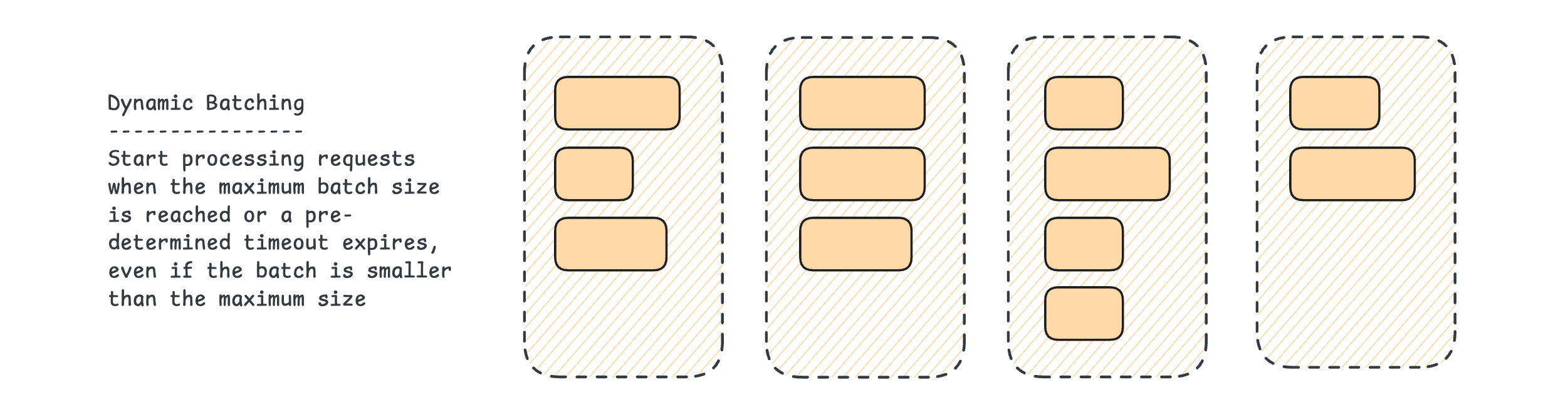
Dynamic batching involves grouping incoming requests and processing them in batches when either the maximum batch size or the maximum wait window is reached.
This means that:
If a batch reaches the maximum size, processing begins immediately.
If the maximum wait window is reached, the processing begins immediately even if the batch contains only one request.
This strategy can handle online inference with unpredictable traffic (variable inter-request intervals), but it still wastes compute, as the GPU must wait for the longest request to finish before returning outputs, even when shorter requests have already finished processing.
3. Continuous batching
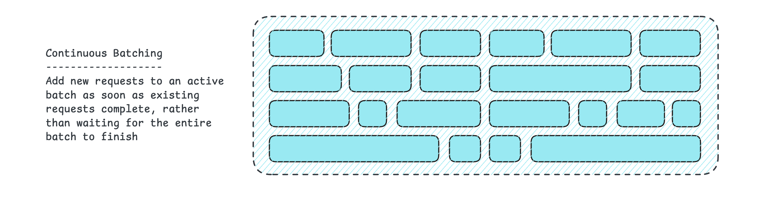
Continuous batching adds and removes incoming requests between decoding iterations. This means a new request can be added to the batch as soon as a request in the batch finishes processing. This substantially minimizes GPU idle time.
It is also called:
In-flight batching because the requests are added and removed on the fly, and
Iteration-level scheduling because the scheduler re-decides the batch membership before every decoding step rather than fixing it once at batch formation
This is one of the most popular strategies in modern high-throughput serving systems that handle massive traffic and can be easily implemented with most serving frameworks such as vLLM, TensorRT-LLM, and SGLang.
Continuous batching treats prefill and decode for requests similarly, even though prefill is compute-bound and decode is memory-bound. This leads us to the next two batching strategies.
4. Continuous batching with chunked prefill
For every request, LLM inference takes place in two phases:
Prefill: The first phase, where all tokens in a user’s prompt are processed together in a single forward pass by the LLM. This phase builds the KV cache and has high arithmetic intensity, making it compute-bound.
Decode: The second phase, where the LLM generates one token at a time, with a single forward pass through the model for each token. This phase has low arithmetic intensity and is memory-bound.
You can read more about these phases using the following links:


Let’s say that user A’s request is in the decode phase (tokens are being generated one at a time) and user B sends a prefill-heavy request with 50,000 tokens. This will cause user A to wait a long time between their generated tokens.
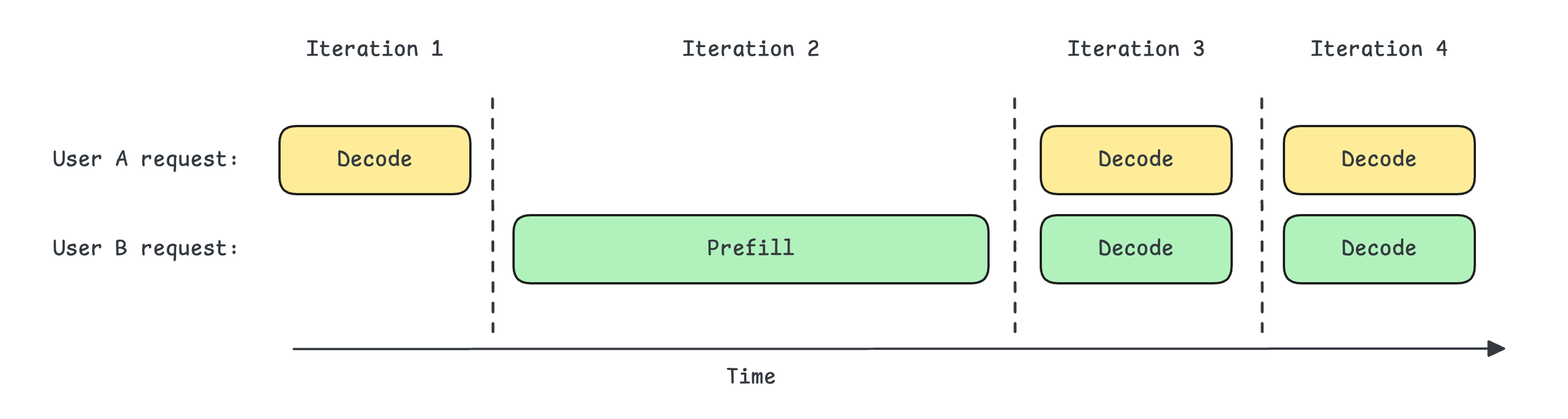
Instead of processing user B’s request all at once, the prefill could be chunked or broken down into smaller token-length pieces and processed with the decode of user A’s request. This ensures that user A continues to receive tokens while user B's long prompt is being processed.
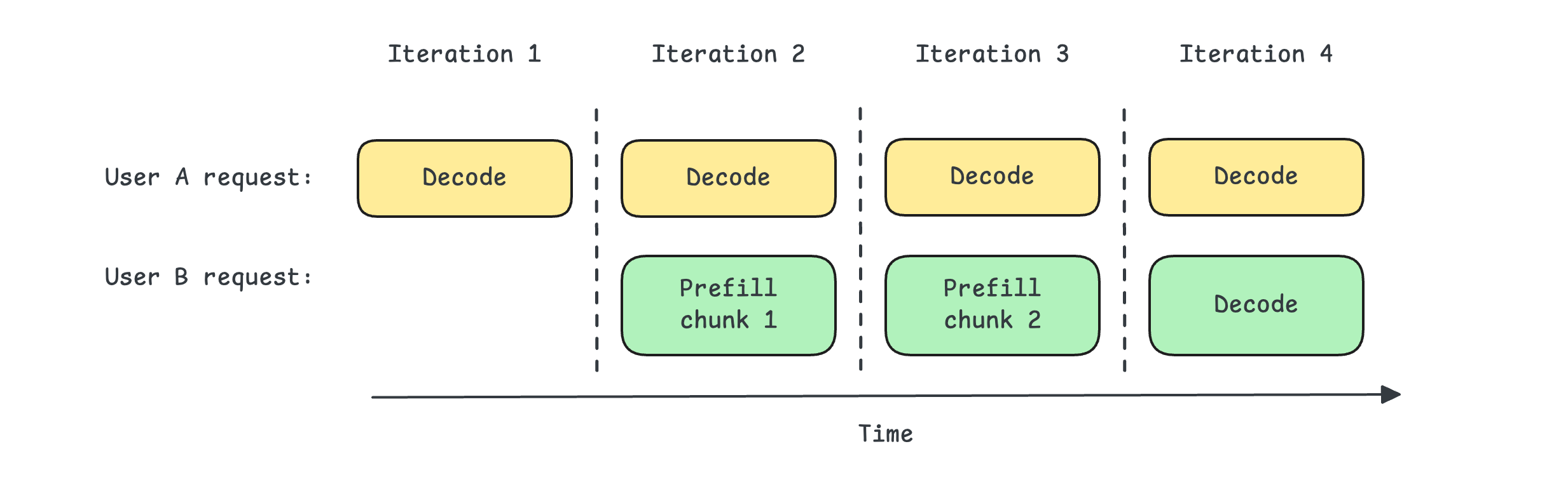
This strategy of chunking prefill is used with continuous batching, which allows processed requests to be added to or removed from the batch between decoding iterations, improving GPU utilization. This is especially beneficial when handling traffic with long-context requests.
One disadvantage of using chunked prefill is that it reduces prefill throughput and increases Time to first token (TTFT) for long prompts. This leads us to the next approach.
5. Prefill-Decode disaggregation
Prefill-Decode disaggregation is a serving architecture that moves the two phases of LLM inference to their dedicated GPU pools.
The dedicated pool of GPUs for prefill is optimized for higher compute, while the dedicated pool of GPUs for decode is optimized for higher memory throughput.
For example, the NVIDIA H200 GPU, compared to the H100, has much faster and larger memory but the same core compute. Therefore, H200s are best used in the decode pool, and H100s in the prefill pool.
During inference, the KV cache is transferred from the prefill-dedicated GPU pool to the decode-dedicated GPU pool. This adds latency and consumes interconnect bandwidth, which is a disadvantage of this architecture at smaller scales. Using high-speed interconnects such as NVLink or InfiniBand helps optimize KV cache transfers.
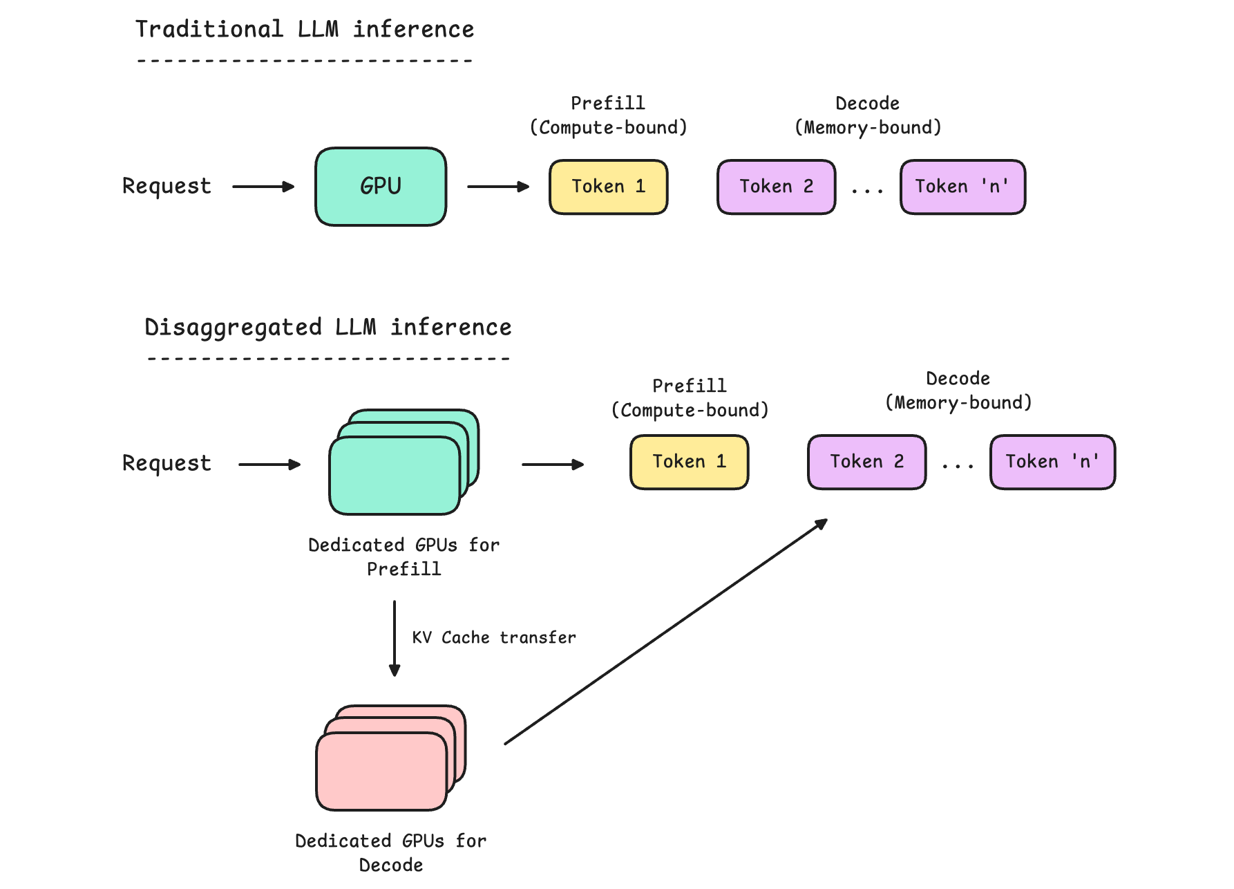
It must be noted that Prefill-Decode disaggregation is a serving architecture in which each GPU pool can still use continuous batching.
Thanks to Pathway, this edition of the newsletter is completely free to read. Show your love by liking, restacking, and sharing it with others! ❤️