
Deep-Diving & Decoding The Secrets That Make DeepSeek So Good
A deep dive into Multi-head Latent Attention (MLA)


DeepSeek is all over the news.
Its models have achieved state-of-the-art performance across multiple benchmarks (educational, factuality, math and reasoning, coding) and are competing head-to-head with OpenAI’s o1.
Since its release, nearly $1 trillion of value has been lost in U.S. technology stocks in the S&P 500.
However, many popular beliefs about it are not correct.
A $6 million training cost for DeepSeek-R1 is being peddled all across the internet, but this is far from the truth (the official figures remain undisclosed).
This figure is actually for the official training of DeepSeek-V3 (the predecessor model for R1) and even then excludes the costs associated with prior research and ablation experiments on architectures, algorithms, or data associated with V3.

Even though the costs are not accurately described, DeepSeek-V3 is still trained with significantly fewer resources than the models of the other prominent players in the LLM market.
But how has this been made possible?
Here’s a story about a groundbreaking architectural change called Multi-Head Latent Attention, which is one reason DeepSeek’s models perform so well at low training resources.
Let’s begin!
We Start Our Journey With ‘Attention’
Attention is a mechanism that allows a model to focus on different parts of the input sequence when making predictions.
The mechanism weighs the importance of each token in the sequence and captures relationships between different tokens of the sequence regardless of their distance from each other.
This helps the model decide which tokens from the input sequence are most relevant to the token being processed.
Attention is not new.
It was popularly introduced for neural machine translation tasks using Recurrent Neural Networks (RNNs).
This version, called the Bahdanau Attention mechanism, uses a bi-directional RNN as an Encoder (bottom blocks in the image) to process input sequences x(1) to x(T) to generate hidden states h(1) to h(T).
The Attention mechanism computes the attention scores for each encoder hidden state, telling how relevant these are to the current decoding step.
These scores are transformed into attention weights a(t,1) to a(t,T)(T is to the total number of input tokens) using the softmax function.
The encoder’s hidden states are weighted according to these and summed to produce a context vector c(t).
At each time step t, the decoder (top blocks in the image) then generates the next output y(t) based on its current hidden state s(t) combined with the context vector c(t), previous hidden state s(t-1) and the previous output y(t-1).

A particular type, called Scaled Dot-Product Attention, was later introduced in the Transformer architecture, which is calculated using the following three values obtained from the input token embeddings:
Query (Q): a vector representing the current token that the model is processing.
Key (K): a vector representing each token in the sequence.
Value (V): a vector containing the information associated with each token.
These are used in the formula as follows:

Transformers use this in three ways:
Self-Attention
This is used in the Transformer’s Encoder.
Here, the Queries, Keys, and Values come from the same input sequence — the previous layer’s output in the Encoder.
2. Masked Self-Attention
This is used in the Transformer’s Decoder.
Here, the Queries, Keys, and Values come from the same sequence — the output sequence generated so far with the future tokens masked.
3. Cross-Attention or Encoder-Decoder Attention
This is used in the Transformer’s Decoder.
Here, the Query comes from the Decoder’s previous layer, while the keys and values come from the Encoder’s output.

Moving Towards Multi-Head Attention
Instead of calculating the Attention score just once, the Transformer runs multiple Attention mechanisms in parallel using multiple heads.
Each head focuses on different aspects of the input sequence (short vs. long-range dependencies, grammatical rules, etc.).
This helps the architecture capture better semantic relationships between different tokens.
Let’s learn how this works.
Let’s say that the Transformer architecture has an overall model dimension represented with d(model) . This represents the dimensionality of the input/ hidden layer representations X.
Instead of working with full-dimensional vectors, each head works with lower-dimensional projections of the Queries, Keys and Values.
These are obtained using learned projection matrices as follows:

The matrices W(Q)(i), W(K)(i), and W(V)(i) projects X into lower-dimensional Query, Key, and Value vectors for each attention head.
d(model) is reduced into smaller dimensions d(k) for Queries and Keys, and d(v) for Values as follows —
d(k) = d(v) = d(model) / hwherehis the number of heads
Next, Scaled dot-product Attention is calculated for each head using its own set of projected Query, Key, and Value matrices.

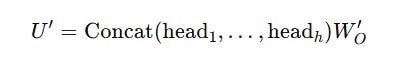
These individual Attention scores are concatenated and linearly transformed using a learned matrix W(O) as shown below.


Going back to the Transformer architecture, it is Multi-head Attention (MHA) that is actually used instead of the basic Attention mechanism (described earlier) for both Self-Attention & Cross-Attention. Also, modern LLMs use only the Decoder part of the Transformer.

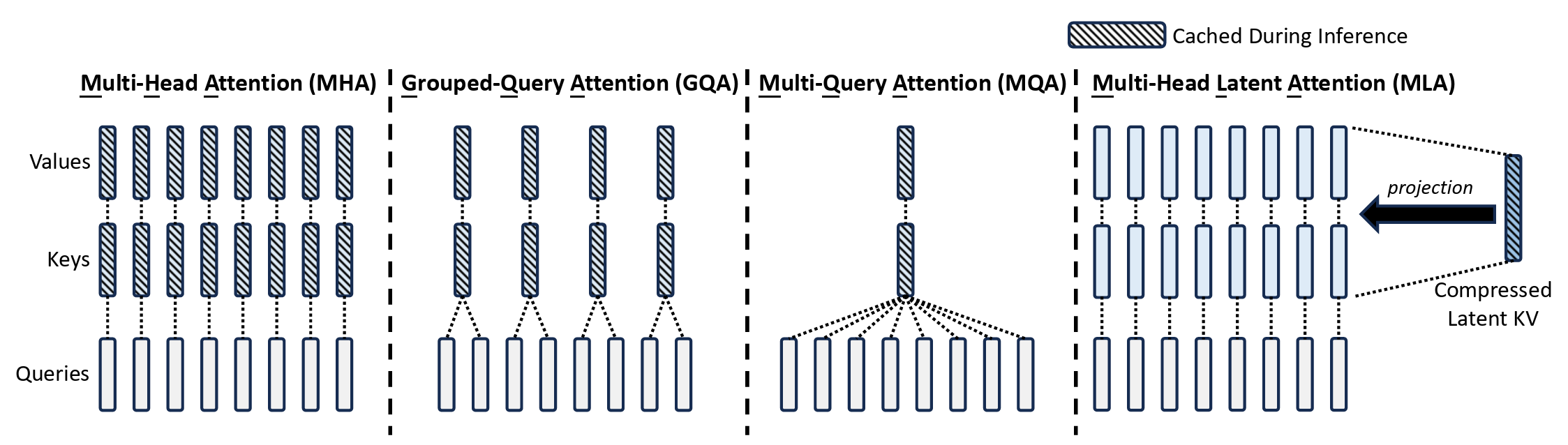
But MHA Is Memory Expensive At Inference
Multi-head Attention (MHA) is a powerful mechanism used by most LLMs today to capture dependencies between tokens, but it causes an issue during inference/ token prediction.
When the LLM generates a token, it must compute the attention scores with all the previous tokens.
Instead of recomputing all keys and values for previous tokens at every time step, they are stored in a Key-Value (KV) Cache.
(Queries are not cached since they are dynamically calculated for each new token, and only Keys and Values need to be reused for future tokens.)
This is a fantastic optimisation step to speed up inference, but as the sequence length increases, the number of stored key-value pairs grows linearly with it.
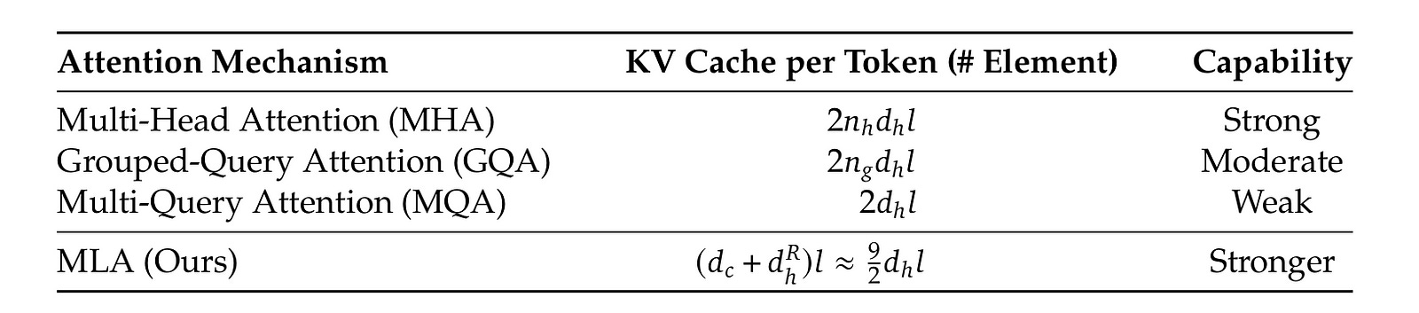
For a transformer with L layers, n(h) heads per layer, and the per-head dimension of d(h), 2 x n(h) x d(h) x Lelements need to be cached for each token.
This is because, for each token, each head independently stores a separate key and value vector of size d(h), and there are n(h) heads per layer and L layers in total.
This cache can become massive over time, especially in long-context models, leading to massive GPU memory usage during cache retrieval and slower inference.
Let’s learn how this memory bandwidth bottleneck is overcome in modern LLMs.
Levelling Up To Multi-Query Attention (MQA)
Unlike traditional Multi-head Attention (MHA), which caches separate key-value pairs per head, Multi-Query Attention (MQA) shares a single set of keys and values across all heads.

This reduces the KV cache size from 2 x n(h) x d(h) x L (as in MHA) to 2 x d(h) x L.
Since only one set of keys and values needs to be fetched, this reduces GPU memory usage, allowing large batch sizes to be processed at inference time.

LLMs like PaLM and Falcon use MQA instead of MHA.
But MQA isn’t perfect.
Since all heads share the same Keys and Values, this reduces effective learned representations, making the LLM less expressive and struggling to track long-range dependencies.
It is also seen that using MQA leads to instability during LLM fine-tuning, particularly with long input tasks.
What’s the fix?
Grouped-Query Attention (GQA) To The Rescue
Published by a team of Google researchers, Grouped-Query Attention (GQA) is a tradeoff between MHA and MQA.
Instead of one KV pair per head (like in MHA) or one KV pair for all heads (like in MQA), GQA groups multiple heads together that share a single KV pair.
Each group processes its own set of queries but shares the same keys and values.
This reduces the KV cache size from 2 x n(h) x d(h) x L (as in MHA) to 2 x d(h) x G, where G is the number of groups.
This makes the inference much faster and, at the same time, allows the LLM to learn its representations effectively.

To summarise —
MHA's generation quality is the best, but its inference speed is the lowest.
MQA leads to the fastest inference speed but the lowest generation quality.GQA balances and interpolates between these two.

Popular LLMs that use GQA in their architecture include Llama 3 series of models, Mistral 7B and DeepSeek LLM (the first version of DeepSeek models).
DeepSeek’s further versions push this performance even more.
Let’s learn how.
Here Comes Multi-Head Latent Attention (MLA)
MLA, or Multi-Head Latent Attention, is built to further reduce the size of the KV cache while still achieving the best performance compared to the previously discussed attention mechanisms (including MHA).
It does this by compressing the KV cache into a lower-dimensional latent space, reducing its size by 93.3%!
Let’s break it down step by step.
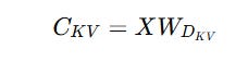
Low-rank Key-Value Joint Compression
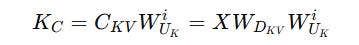
Firstly, instead of computing and storing the Keys and Values for each token, these are compressed into a latent vector C(KV) using a down-projection matrix W(DKV).
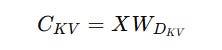
The KV pairs can be reconstructed from this latent vector during inference using per-head up-projection matrices W(UK) (for Keys) and W(UV) (for Values).
To reduce the computational cost:
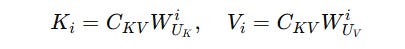
Instead of explicitly calculating the Keys, the matrix
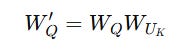
W(UK)is merged intoW(Q)
This is how we were calculating Query and Keys from the latent vector before —
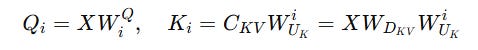
But instead, we redefine the query projection as:
And then compute the Query as:
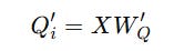
This eliminates the need to explicitly compute K(i) since Q′(i) already includes this information.
Instead of explicitly calculating the Values, the matrix
W(UV)is merged intoW(O)
This is how we calculated the attention for each head and concatenated them:
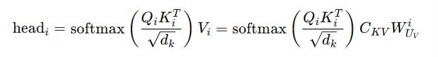
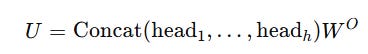
Instead, the output transformation matrix W(O) is merged with W(UV) as follows:
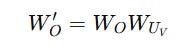
And the final attention output is calculated as:
This eliminates the need to explicitly compute V(i).
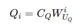
Low-rank Compression For Queries
Similar compression is done for Queries as well.
These are compressed into a latent (compressed) representation C(Q) using a down-projection matrix W(DQ).
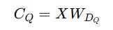
These are reconstructed when needed using an up-projection matrix W(UQ).
This does not reduce the KV cache size but decreases activation memory usage during training.
(Activation memory is the memory used to store intermediate activations during forward propagation in training. These activations are needed for backpropagation to compute gradients.)
During training with MHA, each layer computes and stores Queries explicitly in memory, and this number grows linearly with the number of layers.
Instead, only the compressed representation of the Queries is stored in MLA. This reduces the total activations stored for backpropagation.
To clarify, activations for backpropagation are not stored during inference when the Queries are computed once per token and discarded.
Therefore, compression for Queries only improves training efficiency but keeps the inference performance unchanged.
Researchers try using RoPE to include token position information when using MLA.
However, this is not possible because of how the previous calculations are performed.
To understand why, we must first learn how position encoding works in LLMs.
Positional Encoding — What’s That?
Transformers process tokens in parallel rather than sequentially. This is what gives them the computational advantage over RNNs.
However, this also makes Transformers position-agnostic, meaning they do not have a sense of the order of the tokens they process.
Consider two sentences:
“The cat sits on the mat.”
“The mat sites on the cat.”
To a Transfromer, both of them are the same.
This isn’t good for language processing; therefore, positional information in the form of positional embeddings (vector) is added with token embeddings before Transformers process them.
Positional Embeddings are of two main types:
Absolute Positional Embeddings — where each token is assigned a unique encoding according to its position
Relative Positional Embeddings — where information about how far apart tokens are from each other is encoded rather than their absolute positions
Each of them can be either:
Fixed (calculated using a mathematical function)
Learned (has trainable parameters that are updated with backpropagation during model training)
While relative positional embeddings are popularly used by the T5 Transformer, in the original Transformers paper, the authors use fixed absolute positional embeddings, as shown below.
(Learned positional embeddings are not used in this paper because the fixed embeddings produced nearly identical results.)

For each token position, Positional embeddings (PE) are calculated using alternating sine and cosine functions on even and odd dimensions, respectively.
The denominator 10000 ^ (2i/ d(model)) controls the wavelength of these functions.
This means that for lower dimensions (smaller i), the frequency is high, and the wavelengths are short.
Similarly, for the higher dimensions (larger i), the frequency is low, and the wavelengths are long.
These wavelengths form a Geometric progression, with the smallest and the largest values being 2π and 10000 × 2π , respectively.
This makes the model capture the short-term and long-term dependencies in the input sequence using the high and low frequencies, respectively.
Since the dimensions of these Positional Embeddings are the same as the token embeddings, they can be directly summed as follows before being passed to the Transformer to process.

These embeddings can also capture the relative relationships between tokens, as their positional embeddings are related linearly.
Improving Learning Further With RoPE
Previous embedding approaches can struggle to capture dependencies in sequences longer than those seen during training.
These approaches also add positional embeddings to the token embeddings, which increases the total parameters and complexity, leading to increased computational training costs and slower inference.
A 2023 research introduced a new way of directly encoding both absolute and relative positions in the attention mechanism.
Their method is called Rotary Position Embedding or RoPE.
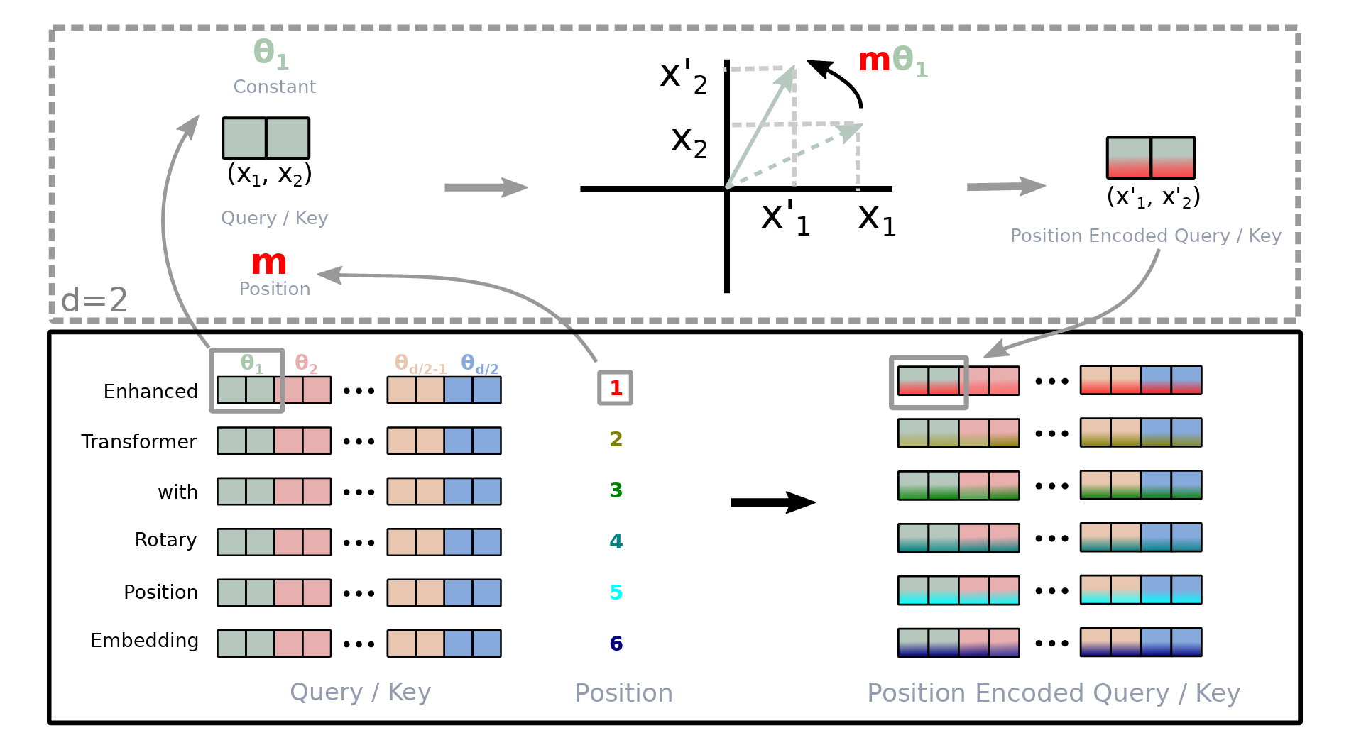
Instead of adding position embeddings, as in the previous approaches, RoPE rotates the token embeddings according to their positions.
For a token embedding x(m) of dimension d at position m, it is transformed into Query (q(m)) and Key (k(n)) vectors as follows using weight matrices W(q) and W(k), respectively.

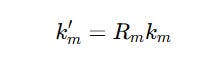
RoPE rotates these vectors before they are used in the self-attention calculation. This is done using a position-dependent rotation matrix R(m).

R(m) acts independently on each pair of dimensions in q and k.
For a case where these vectors are two-dimensional (d = 2), the rotation matrix R(m) is defined as:

This 2D rotation matrix rotates these vectors counter-clockwise, proportional to their position m by an angle of mθ where θ is a constant (1 in the case of d = 2).
For a two-dimension query vector q(m) = (q1, q2) , this transformation will result in:


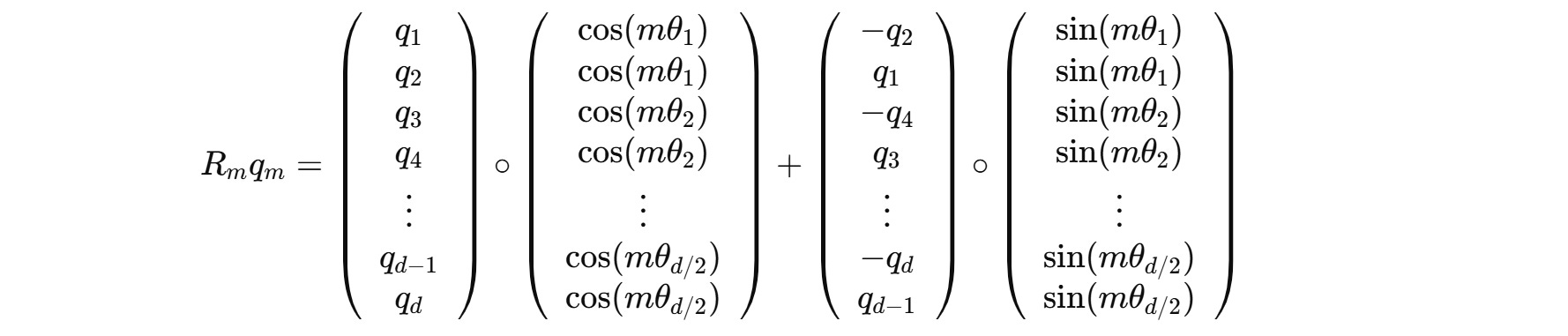
But query and key vectors are usually higher-dimensional (assumed an even number of dimensions), and to work with them, they are paired and separate 2D rotations are applied to each adjacent pair of dimensions.
For example, for a 4-dimension query vector q(m) = (q1, q2, q3, q4), two independent rotations are applied for (q1, q2) and (q3, q4) as shown below.

These can be expanded to:


The angle of rotation θ(i) for each pair of dimensions is different and is calculated as follows:

This ensures that the low-frequency rotations for higher dimensions capture long-range dependencies and the high-frequency rotations for lower dimensions capture short-term dependencies.
This θ is similar to what we learned when describing the sinusoidal embeddings from the original Transformers paper.
The overall rotation matrix for higher dimensions looks as follows.

One can avoid explicit matrix multiplication to make the process of computing the rotated queries and keys computationally efficient.
This can be done by precomputing cos(mθ(i)) and sin(mθ(i)) for each position m, and then performing simple element-wise multiplications and additions between the terms.
For example, this is how we calculated the rotated query q’(m) previously:


This can be changed to:

The complete calculation is shown below:
Next, the self-attention score is calculated as the dot product between the rotated queries and keys as follows:

Since the rotation matrices can be written as follows,

The equation becomes:

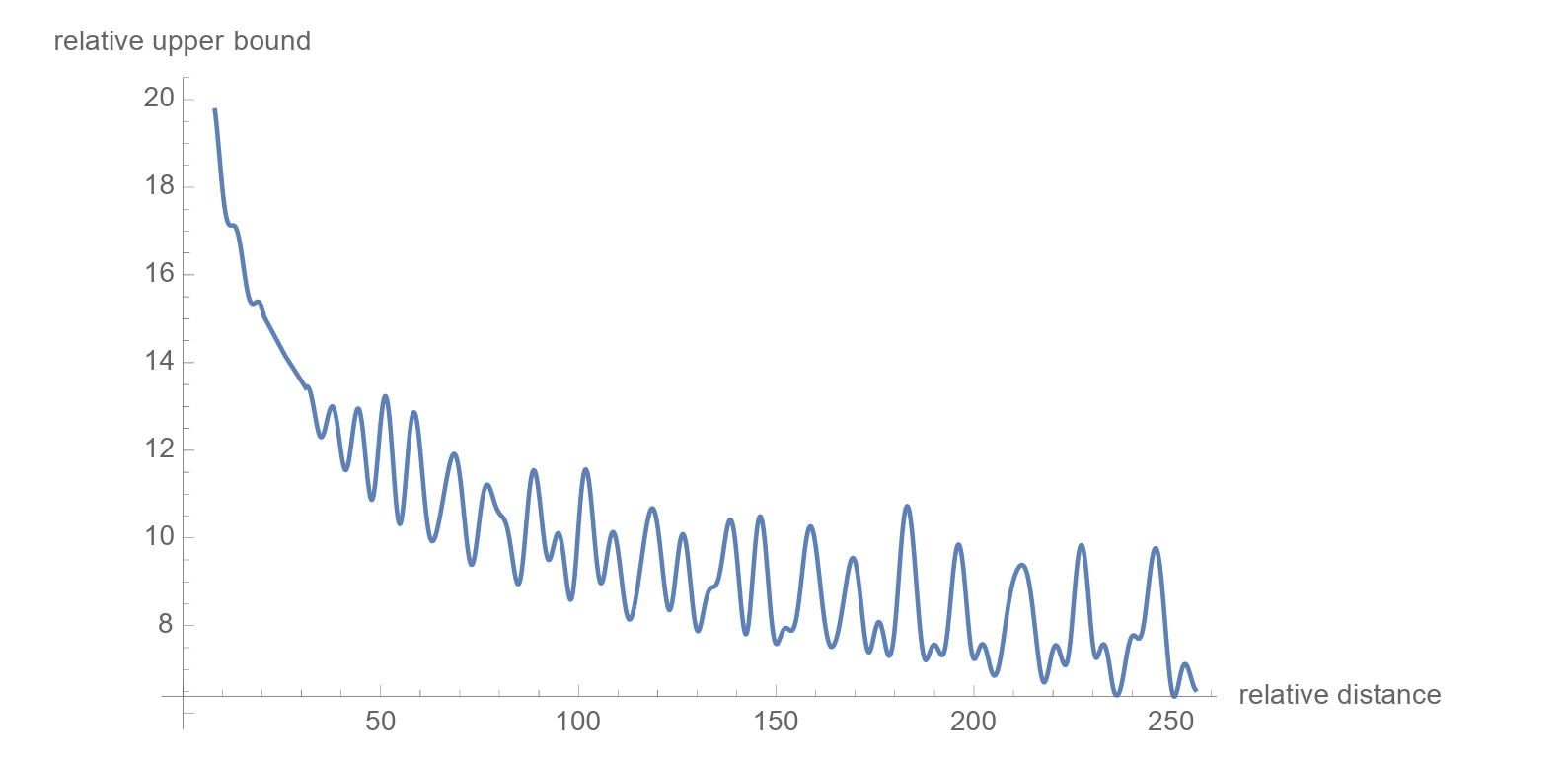
Thanks to RoPE, the attention score now encodes the relative position of tokens (n − m) without needing additional relative embeddings.
There’s another cool property of these embeddings: the relative importance of the connection between far-apart tokens is lower than closer ones.
The mathematical explanation of this can be found in the research paper, and curious readers are encouraged to check it out.
Now that we know how RoPE works, we need to figure out a way to apply it to MLA.
Why Is RoPE Incompatible With MLA?
Returning to MLA, we first created a latent compressed representation of the keys and values C(KV) to reduce memory usage and improve inference efficiency.
We know that RoPE involves rotating queries and keys according to positional information using the rotation matrix R(m) before calculating the attention scores:
However, since MLA stores the compressed key-value cache rather than full keys, applying RoPE will mean that all previous keys must be recomputed every time a new token is generated.
This breaks the efficiency achieved by using the compressed KV representation in the first place.
Then there’s another issue.
Remember how, instead of recalculating the keys during inference, the key up-projection matrix W(UK) was merged into W(Q) for optimization?
If we apply RoPE after key reconstruction as follows:

This prevents the merging because matrix multiplication is not commutative.

Thus, W(UK) cannot be decoupled and merged with W(Q) as done originally.
How Is RoPE Used In MLA Then?
In MLA, a new approach to applying RoPE called Decoupled Rotary Position Embedding is introduced.
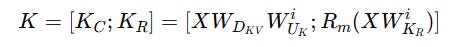
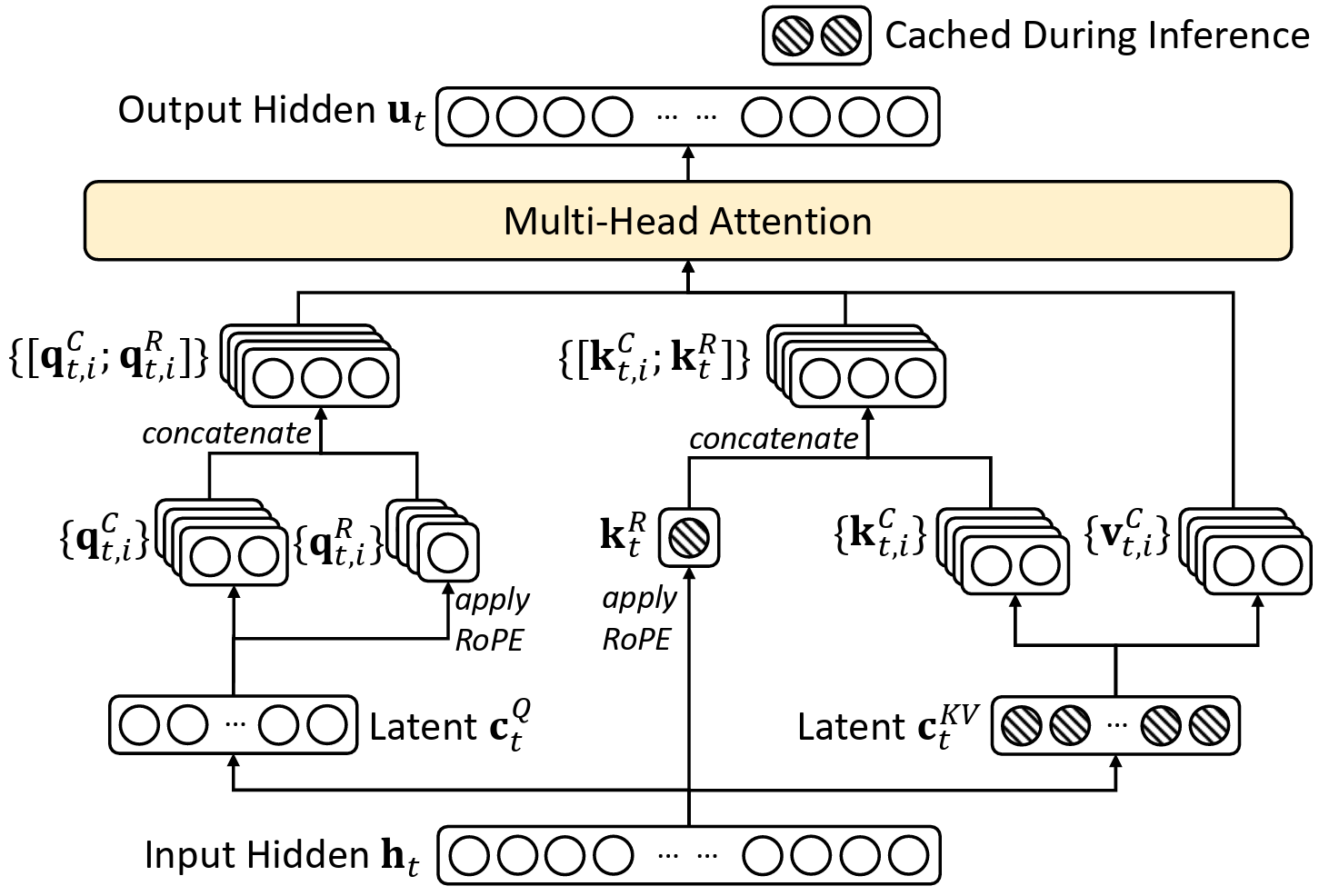
Firstly, two types of keys are calculated:
Latent keys
K(C)that are compressed keys calculated like we previously discussed.
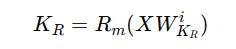
2. Position-sensitive or Decoupled keys K(R) that are non-compressed keys that store the position information required to apply RoPE as follows:
Both of these are concatenated and shown below.
The same operations are performed for queries as well.
This results:
Latent queries
Q(C)

2. Position-sensitive or Decoupled queries Q(R) for RoPE

Both of these are concatenated and are shown below.

These are calculated at inference and not stored.
The approach gives us the best of both worlds, where we still benefit from low-rank KV compression while K(R) can be stored separately and allows the application of position-sensitive transformations without breaking the attention calculations with RoPE.
In this approach, we cache K(R) and C(KV) and a total of [d(c) + d(h)(R)] x L elements per token need to be cached where d(c) is the latent key dimension, d(h)(R) is the per-head dimension of decoupled keys and L is the number of layers in MLA.
This is much more efficient than for a transformer with L layers, n(h) heads per layer, and the per-head dimension of d(h), where 2 x n(h) x d(h) x Lelements need to be cached for each token.
Finally, the attention score is calculated using both compressed and position-sensitive queries and keys:

The final output is calculated as follows (where V(C) is retrieved dynamically from the key-value cache C(KV)):

You must note that although these explicit calculations are shown to clarify the process, keys and values are never explicitly calculated, as we previously discussed.
The complete MLA architecture is shown below.
How Good Is MLA?
MLA stores a small number of elements in its KV cache, which is equal to GQA with only 2.25 groups but can achieve stronger performance than MHA.
When a dense model with 7B total parameters is trained with different attention mechanisms, MHA performs significantly better than both GQA and MQA on the tested benchmarks.
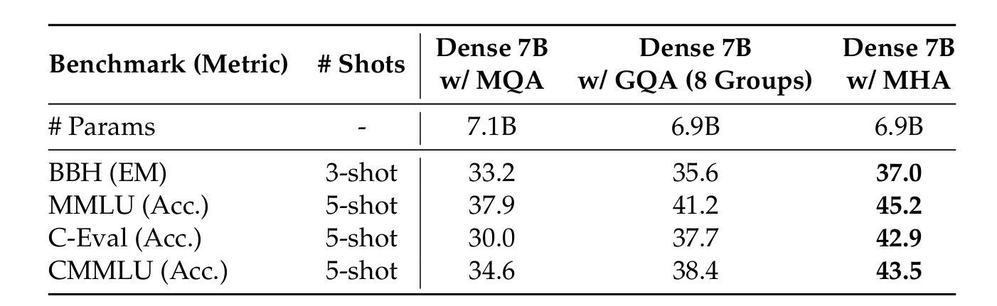
This shows that GQA and MQA trade off some performance to reduce the Key-Value (KV) cache size.
But here’s the surprising part!
When two MoE models (with 16B and 250B total parameters) trained with different attention mechanisms are evaluated, it is seen that MLA outperforms MHA across most benchmarks.
This performance is achieved combined with a significantly smaller KV cache, with a 14% KV cache usage for the small MoE model and a 4% KV cache usage for the large MoE model trained with MLA than MHA.
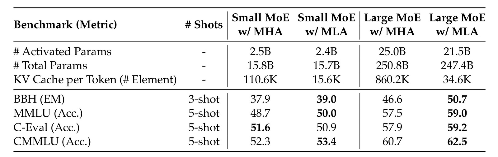
MLA does not trade off performance for the reduction in KV cache; instead, it improves performance and efficiency at the same time.
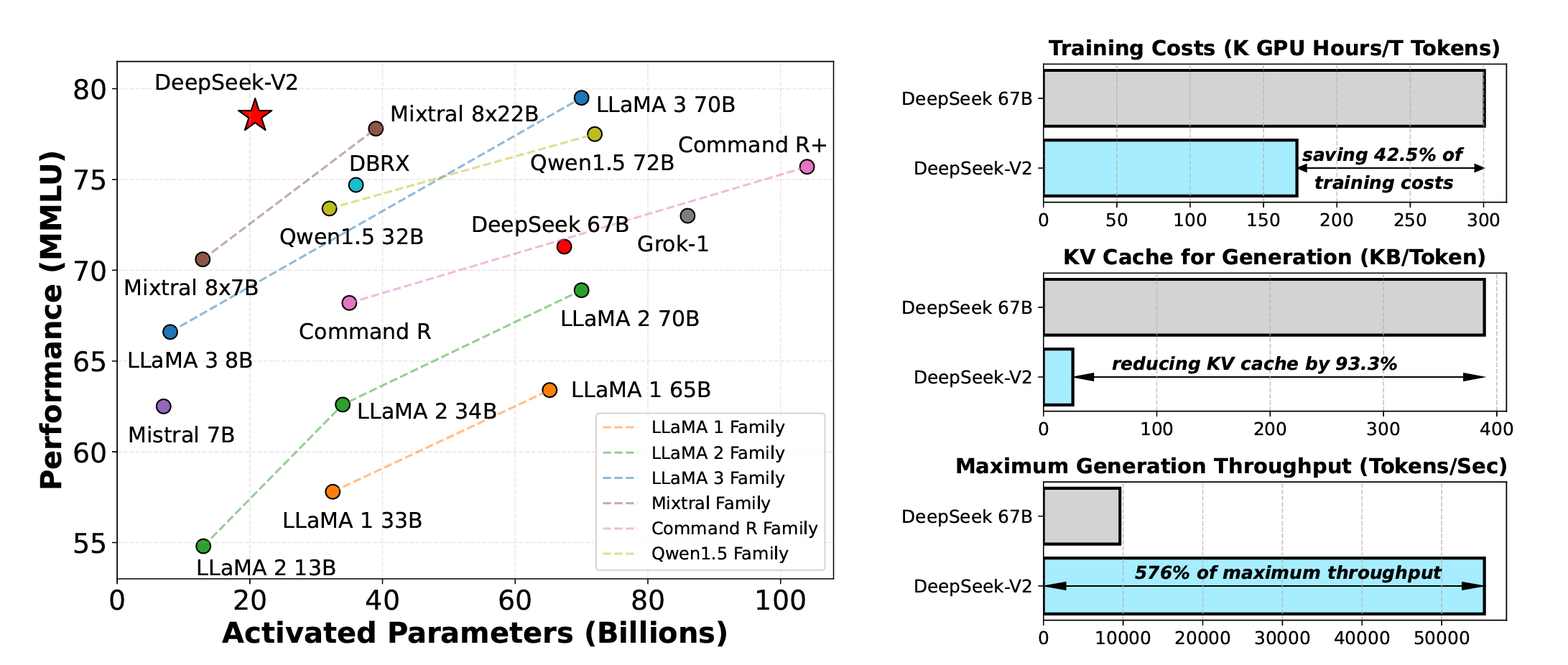
The following image shows how MLA is one of the reasons for the improvement in the MMLU performance, reduced training costs and size of the KV cache and improved generation throughput of DeepSeek-V2 compared to DeepSeek 67B.
(Note that DeepSeek 67B is the first LLM from DeepSeek, which is a dense model (as opposed to MoE) that uses Grouped-Query Attention (GQA) with RoPE embeddings (as opposed to MLA) trained on lesser tokens and less sophisticated training methodologies.)
MLA is also one of the reasons why DeepSeek-V3 performs so well on diverse language, coding and mathematics benchmarks.
That’s everything for Multi-Head Latent Attention (MLA).
Stay tuned for upcoming articles in this series, where we dive deep into the other architectural and training modifications that make DeepSeek models perform well.
Thanks for reading!
Source Of Images
All images are obtained from the DeepSeek-V2 research paper unless stated otherwise.
Further Reading
Research paper titled ‘DeepSeek-V3 Technical Report’ published in ArXiv
Research paper titled ‘Fast Transformer Decoding: One Write-Head is All You Need’ published in ArXiv