
Build a Decoder-only Transformer from Scratch
Build a Decoder-Only Transformer, the core architecture powering GPT-like LLMs from scratch in PyTorch.

In the previous lesson on ‘Into AI’, we learned how to implement the Causal Multi-Head Self-Attention.

Honestly, it is one of the most challenging parts of the LLM architecture to understand.
What comes after it is extending it and building a complete Decoder-Only Transformer that powers an LLM. This lesson is all about that.
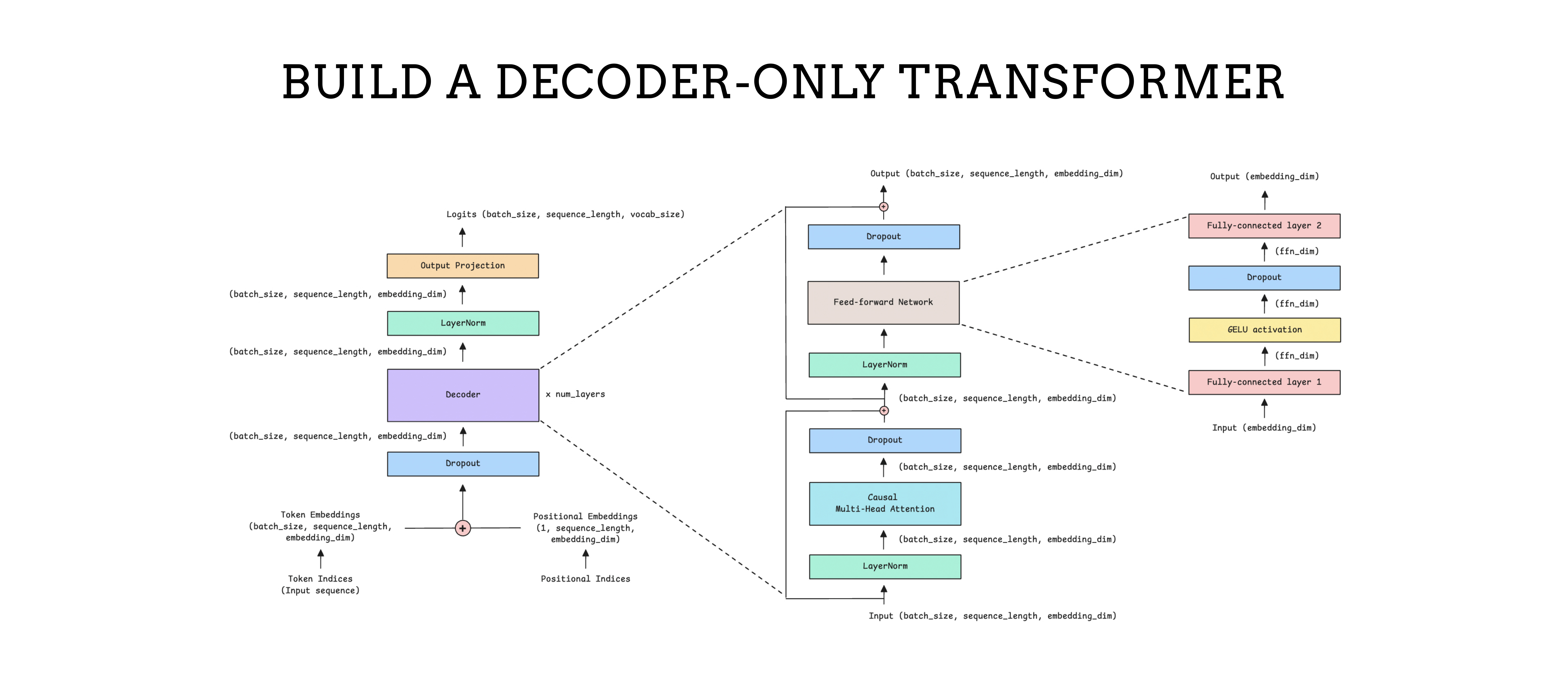
Before we start, I want to introduce you to my book, ‘LLMs In 100 Images’.
It is a collection of 100 easy-to-follow visuals that explain the most important concepts you need to master to understand LLMs today.
What is the Decoder-only Transformer?
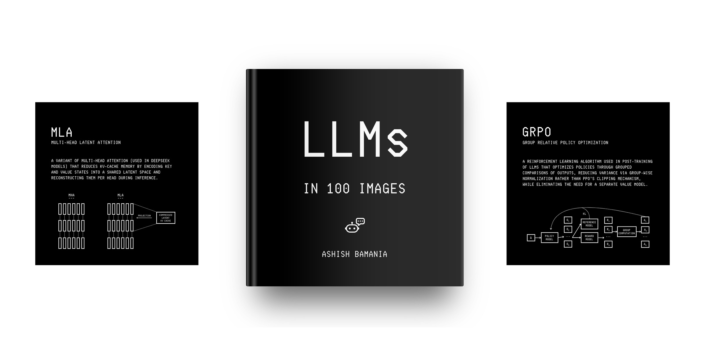
The original Transformers paper, titled “Attention is all you need,” introduced the Encoder-Decoder Transformer architecture. This architecture is well-suited for the language translation task.
Modern LLMs like GPT and Llama use the Decoder-only transformer architecture (shown on the right in the above image). This is much better suited to text generation.
Its components are as follows:
Causal (or Masked) Multi-Head Self-Attention
Feed-Forward Network (FFN)
Layer Normalization
Residual or Skip connections
We have already learned to implement the Causal Multi-Head Self-Attention (see code below), so let’s move on to learn about the other components, starting with the feed-forward network.
import torch
import torch.nn as nn
import math

class CausalMultiHeadSelfAttention(nn.Module):
  def __init__(self, embedding_dim, num_heads):
    super().__init__()

    # Check if embedding_dim is divisible by num_heads
    assert embedding_dim % num_heads == 0, "embedding_dim must be divisible by num_heads"

    # Embedding dimension
    self.embedding_dim = embedding_dim

    # Number of total heads
    self.num_heads = num_heads

    # Dimension of each head
    self.head_dim = embedding_dim // num_heads

    # Linear projections for Q, K, V (to be split later for each head)
    self.W_q = nn.Linear(embedding_dim, embedding_dim, bias = False)
    self.W_k = nn.Linear(embedding_dim, embedding_dim, bias = False)
    self.W_v = nn.Linear(embedding_dim, embedding_dim, bias = False)

    # Linear projection to produce final output
    self.W_o = nn.Linear(embedding_dim, embedding_dim, bias = False)

  def _split_heads(self, x):
    """
    Transforms input embeddings from
    [batch_size, sequence_length, embedding_dim]
    to
    [batch_size, num_heads, sequence_length, head_dim]
    """
    batch_size, sequence_length, embedding_dim = x.shape

    # Split embedding_dim into (num_heads, head_dim)
    x = x.reshape(batch_size, sequence_length, self.num_heads, self.head_dim)

    # Reorder and return the intended shape
    return x.transpose(1,2)

  def _merge_heads(self, x):
    """
    Transforms inputs from
    [batch_size, num_heads, sequence_length, head_dim]
    to
    [batch_size, sequence_length, embedding_dim]
    """
    batch_size, num_heads, sequence_length, head_dim = x.shape

    # Move sequence_length back before num_heads in the shape
    x = x.transpose(1,2)

    # Merge (num_heads, head_dim) back into embedding_dim
    embedding_dim = num_heads * head_dim
    x = x.reshape(batch_size, sequence_length, embedding_dim)

    return x

  def forward(self, x):
    batch_size, sequence_length, embedding_dim = x.shape

    # Compute Q, K, V
    Q = self.W_q(x)
    K = self.W_k(x)
    V = self.W_v(x)

    # Split them into multiple heads
    Q = self._split_heads(Q)
    K = self._split_heads(K)
    V = self._split_heads(V)

    # Calculate scaled dot-product attention
    attn_scores = Q @ K.transpose(-2, -1)

    # Scale
    attn_scores = attn_scores / math.sqrt(self.head_dim)

    # Apply causal mask (prevent attending to future positions)
    causal_mask = torch.tril(torch.ones(sequence_length,
    sequence_length, device=x.device)) # Create lower triangular matrix

    causal_mask = causal_mask.view(1, 1, sequence_length,
    sequence_length)  # Add batch and head dimensions

    attn_scores = attn_scores.masked_fill(causal_mask == 0,
    float("-inf")) # Mask out future positions by setting their scores
    to -inf

    # Apply softmax to get attention weights
    attn_weights = torch.softmax(attn_scores, dim = -1)

    # Multiply attention weights by values (V)
    weighted_values = attn_weights @ V

    # Merge head outputs
    merged_heads_output = self._merge_heads(weighted_values)

    # Final output
    output = self.W_o(merged_heads_output)

    return output
The Feed-Forward Network
While the role of the Causal Multi-Head Self-Attention block is to understand inter-token relationships in the input sequence, the Feed-forward network (FFN) helps learn token-wise patterns well by:
Processing each token independently of the others
Expanding dimensionality of token embeddings to increase representational capacity
Adding non-linearity to inputs using activation functions like GELU/ ReLU
Projecting them back to the original embedding dimension before passing them to the next layer
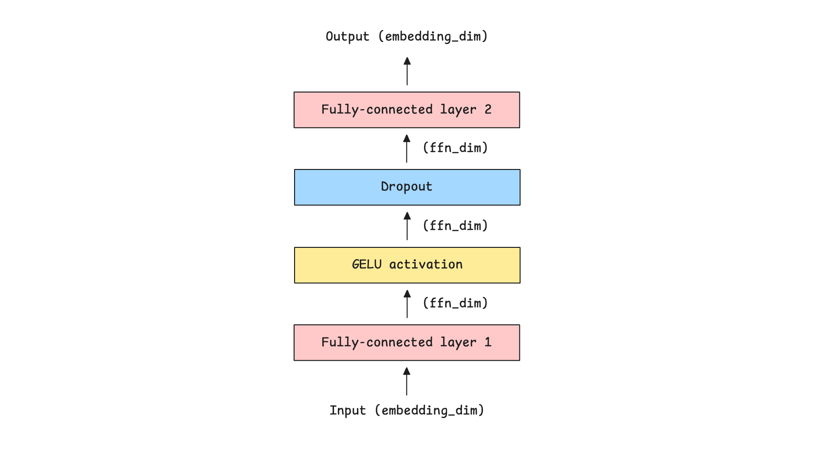
Let’s implement a 2-layer FFN in PyTorch.
class FeedForwardNetwork(nn.Module):
  def __init__(self, embedding_dim, ff_dim, dropout = 0.1):
    super().__init__()

    self.fc1 = nn.Linear(embedding_dim, ff_dim) # Expand feature space
    to ff_dim (dimension of FFN)

    self.activation = nn.GELU() # Introduce non-linearity

    self.fc2 = nn.Linear(ff_dim, embedding_dim) # Project back to
    embedding_dim (original embedding dimension)

    self.dropout = nn.Dropout(dropout) # Regularization with Dropout

  def forward(self, x):
    x = self.fc1(x)
    x = self.activation(x)
    x = self.dropout(x)
    x = self.fc2(x)

    return x
These operations are shown visually along with the input and output dimensions for each layer, as follows.
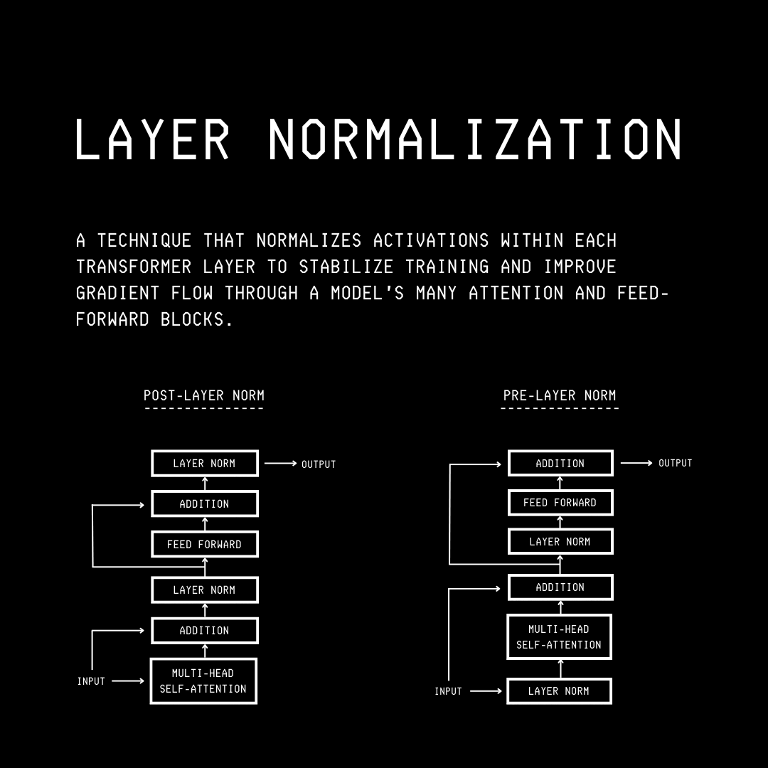
Layer Normalization
Layer Normalization or LayerNorm normalizes each token’s feature vector to zero mean and unit variance, then applies learned scaling and shifting.
This stabilizes and speeds up training by keeping each token’s representation well-scaled and gradients numerically stable as it flows through the layers of a Transformer.
There are two ways in which LayerNorm is used:
Post-LayerNorm (Post-LN), where LayerNorm is applied after each sublayer as in the original Transformer paper
Pre-LayerNorm (Pre-LN), where LayerNorm is applied before each sublayer, as in modern architectures like GPT and Llama, leading to more stable gradients during training. We will implement Pre-LN in our decoder-only transformer.
For a more detailed discussion on Normalization, please refer to the following lesson.

Residual Connections
A Residual or Skip connection adds the input of a layer directly to its output, bypassing the layer.
Such connections help information and gradients flow through deep networks, making training more stable and effective.

The Decoder Block
Now that we understand the individual components, let’s use them to create a Decoder block.
This is how it looks, along with the input and output dimensions for each layer.
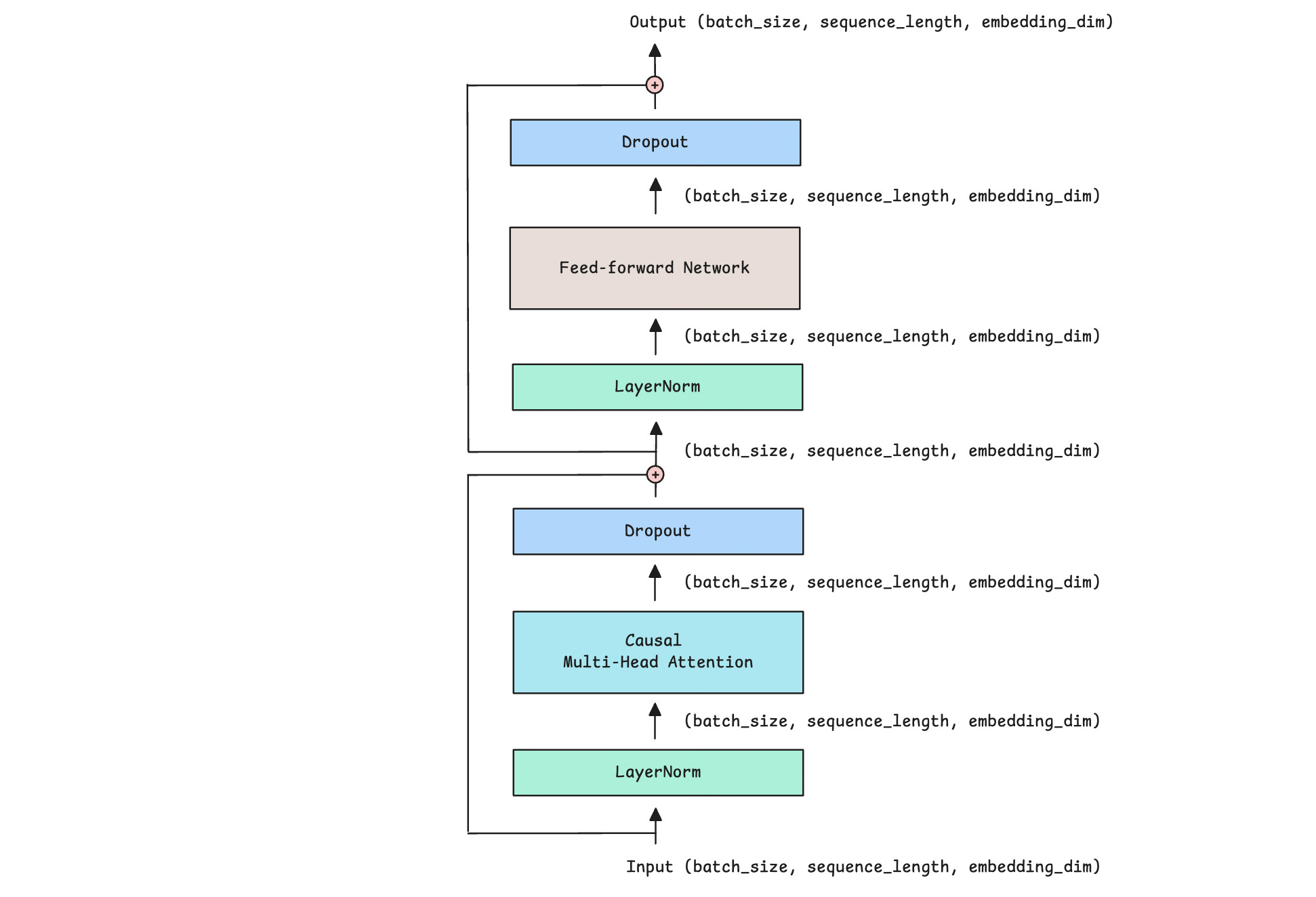
Let’s implement it in PyTorch.
class Decoder(nn.Module):
def __init__(self, embedding_dim, ff_dim, num_heads, dropout=0.1):
super().__init__()
self.attention = CausalMultiHeadSelfAttention(embedding_dim,
num_heads)
self.ffn = FeedForwardNetwork(embedding_dim, ff_dim, dropout)
# LayerNorm is applied before each sublayer (Pre-LN)
self.ln1 = nn.LayerNorm(embedding_dim)
self.ln2 = nn.LayerNorm(embedding_dim)
# Dropout applied to sublayer outputs for regularization
self.dropout = nn.Dropout(dropout)
def forward(self, x):
# Causal MHA
attention_output = self.attention(self.ln1(x))
# Residual connection
x = x + self.dropout(attention_output)
# Feed-forward network
ffn_output = self.ffn(self.ln2(x))
# Residual connection
x = x + self.dropout(ffn_output)
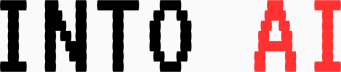
return xThe Decoder-only Transformer
Next, we will stack multiple Decoder blocks to create the complete Decoder-only Transformer model.
The following image shows what it looks like.
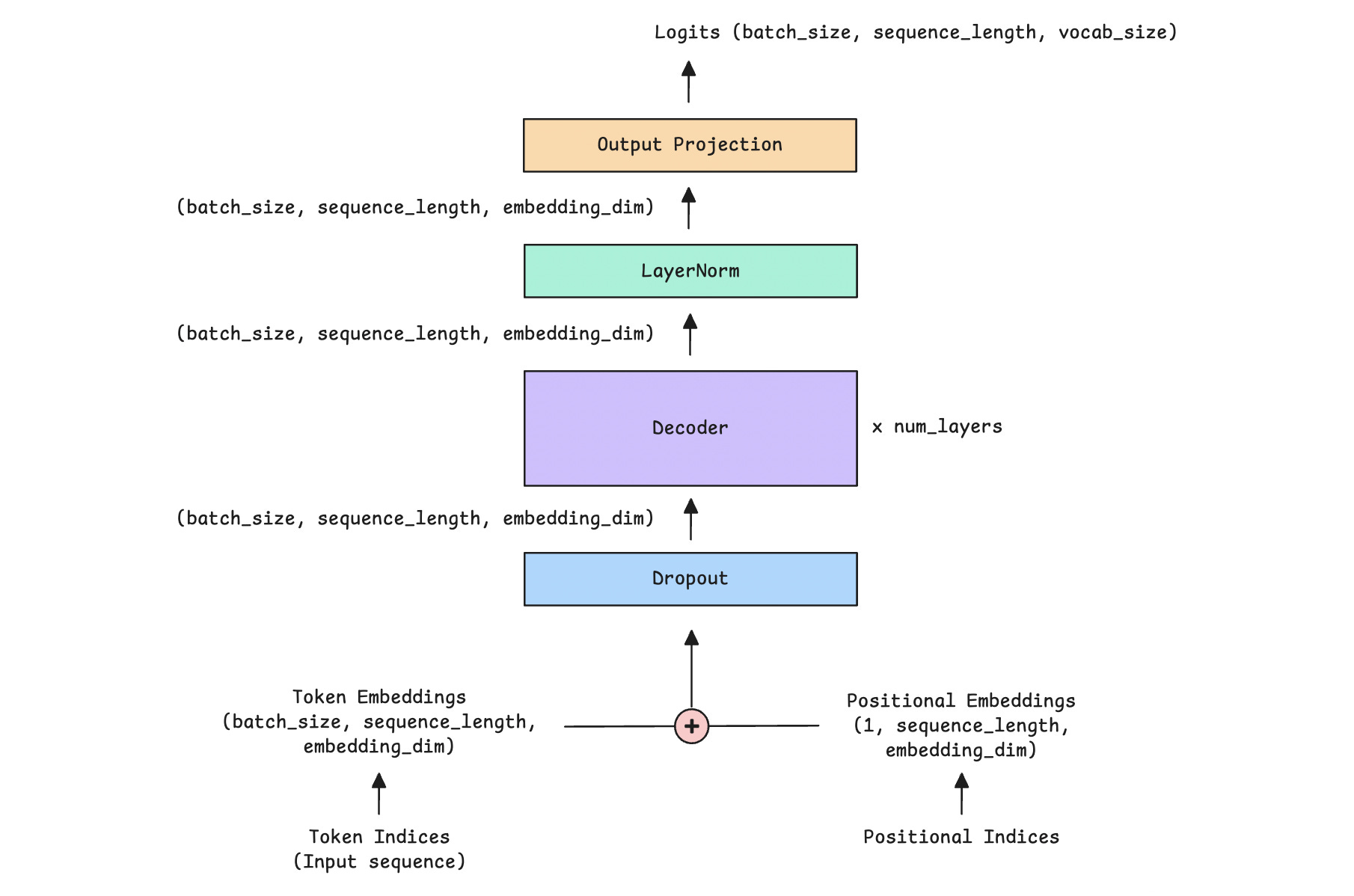
The Decoder is further expanded and shown in the image below.
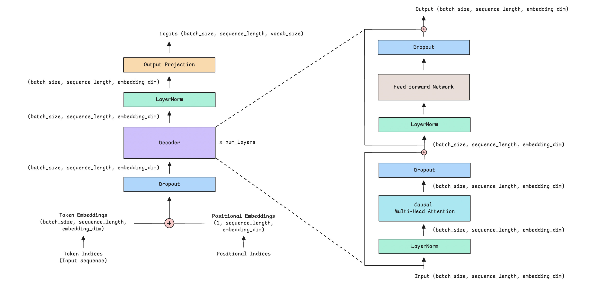
Let’s understand the operations taking place in the Decoder-only Transformer.
We start with an input sequence that contains token indices. These indices are integers that represent tokens (words or subwords) in a vocabulary.
The vocabulary is the complete list of all tokens a model knows. It is implemented as a dictionary where each token is mapped to a unique integer ID.
A sample vocabulary could look like.
vocab = {
    "the": 1,
    "a": 2,
    # ...
    "man": 34,
    "woman": 35,
    # ...
    "eats": 42,
    # ...
    "lunch": 192,
    # ...
}
A sample input sequence, “the man eats lunch,” will be represented as a list of token indices: [1, 34, 42, 192].
These token indices are converted into token embeddings and combined with positional embeddings, which provide the model with information about each token's position in the sequence.
In our example with token indices [1, 34, 42, 192], their positions are represented by [0, 1, 2, 3]. These are converted into token embeddings and positional embeddings and added together before passing to the model.
(For the more curious ones, we are using learned absolute positional embeddings here. A detailed lesson on positional embeddings and RoPE can be found using this link.)
These are passed through stacked decoder blocks (with self-attention and feedforward layers) and normalized using layer normalization.
Finally, an output projection (a Linear layer) projects these inputs to the vocabulary size, producing logits for each predicted next token.
Logits are the raw, unnormalized scores the model outputs for each token in the vocabulary.
We apply softmax to convert the logits into probabilities, then select the highest-scoring token for text generation.
Let’s implement these operations in PyTorch.
class DecoderOnlyTransformer(nn.Module):
    def __init__(self, vocab_size, embedding_dim, num_heads, ff_dim,
                 num_layers, max_seq_length, dropout = 0.1):
        super().__init__()

        self.embedding_dim = embedding_dim
        self.max_seq_length = max_seq_length

        # Token embeddings
        self.token_embedding = nn.Embedding(vocab_size, embedding_dim)

        # Positional embeddings
        self.positional_embedding = nn.Embedding(max_seq_length,
        embedding_dim)

        # Dropout
        self.dropout = nn.Dropout(dropout)

        # Stack of Decoder blocks
        self.decoders = nn.ModuleList([
            Decoder(embedding_dim, ff_dim, num_heads,
        dropout) for _ in range(num_layers)
        ])

        # LayerNorm
        self.final_ln = nn.LayerNorm(embedding_dim)

        # Output projection to vocabulary
        self.output_proj = nn.Linear(embedding_dim, vocab_size)

    def forward(self, x):
        # x represents token indices
        batch_size, seq_length = x.shape

        # Create positional indices
        # Unsqueeze(0) adds a new dimension at position 0 allowing
        positional embeddings to be broadcast across the batch
        positions = torch.arange(0, seq_length, device =
        x.device).unsqueeze(0)

        # Create token embedding
        token_embedding = self.token_embedding(x)

        # Create positional embedding
        positional_embedding = self.positional_embedding(positions)

        # Combine embeddings and add Dropout
        x = self.dropout(token_embedding + positional_embedding)

        # Forward pass through decoder blocks
        for decoder in self.decoders:
          x = decoder(x)

        # Apply LayerNorm to the output
        x = self.final_ln(x)

        # Output projection to vocabulary to get logits
        logits = self.output_proj(x)

        return logits
Inference from the Decoder-only Transformer
It’s time to define the hyperparameters and instantiate our Decoder-only transformer model.
# Hyperparameters

vocab_size = 50257
embedding_dim = 768
ff_dim = 3072  # 4 × embedding_dim
num_heads = 12
num_layers = 12
max_seq_length = 1024
batch_size = 2
sequence_length = 128
# Create model
model = DecoderOnlyTransformer(
vocab_size=vocab_size,
embedding_dim=embedding_dim,
num_heads=num_heads,
ff_dim=ff_dim,
num_layers=num_layers,
max_seq_length=max_seq_length,
dropout=0.1
)Next, we create an input sequence to pass to the model.
In real training or inference, the input sequences are generated by tokenizing actual data, but for this tutorial, we will initialize an input sequence with random values.
# Sample input sequence with token indices
# 2D tensor of shape (batch_size, sequence_length) of random integer token IDs
input_tokens = torch.randint(0, vocab_size, (batch_size, sequence_length))
Let’s run a forward pass of the input sequence through our model and get an output.
# Forward pass
output = model(input_tokens)
The shapes of the input and the model's output are as follows.
print(f"Input shape: {input_tokens.shape}")
# Input shape: torch.Size([2, 128]) # (batch_size, sequence_length)

print(f"Output shape: {output.shape}")
# Output shape: torch.Size([2, 128, 50257]) # (batch_size, sequence_length, vocab_size)
The output contains logits for all positions in the input sequence.
To generate the next token from the input sequence, we obtain the logits for the last position.
We convert these logits into a probability distribution using softmax, where higher logits correspond to higher probabilities and all probabilities sum to 1.
Finally, we use the argmax method to select the token with the highest probability (greedy decoding). This gives us the predicted next token index for each sequence in the batch.
# Generate next token

with torch.no_grad(): # Disable tracking gradients (no backpropagation)
    last_logits = output[:, -1, :]  # Logits for last position only

    last_probs = torch.softmax(last_logits, dim=-1) # Convert to
    probabilities

    next_token = torch.argmax(last_probs, dim=-1) # Pick highest
    probability token (Greedy decoding)

    print(f"Predicted next token indices: {next_token}")
    # Predicted next token indices: tensor([2638, 12880])

    print(f"Next token shape: {next_token.shape}")
    # Next token shape: torch.Size([2]) # (batch_size)
There are many other decoding strategies for generating text from LLMs. Here is a detailed lesson on them.

Note that we have not trained our model, and its weights are randomly initialized, so these outputs are random and meaningless. We will discuss model training in a separate lesson.
That’s everything for this article. Thanks for reading it!
If you are struggling to understand this article well, start here:


Share this article with others, and if you want to get even more value from this publication, consider becoming a paid subscriber for just $50/ year.
You can also check out my books on Gumroad and connect with me on LinkedIn to stay in touch.

Brilliant walkthrough on the decoder architecture. The way you broke down pre-LayerNorm vs post-LayerNorm makes way more sense now, i always wondered why modern LLMs switched to Pre-LN. When I was implementing transformres last year I kept getting gradient issues and didnt realize the LayerNorm placement was key. Really appreciate the dimension tracking alongside the code too.