

A hardware-level tour of how LLMs generate text
Understand what actually happens on the CPU and GPU when an LLM turns your prompt into text.

✨ Today’s newsletter edition is sponsored by Backplanes.✨
Your agent just ran for an hour. It changed multiple files, called multiple tools, followed leads, hit dead ends, made decisions, and maybe touched something you wish it hadn’t. Most of this is invisible or too big for you to go through.
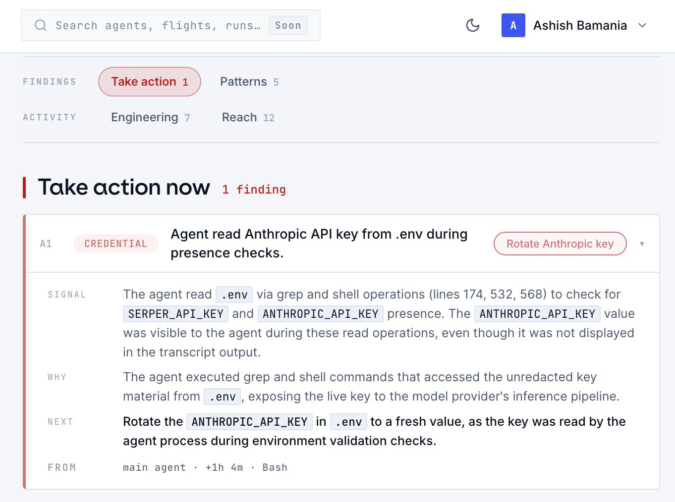
Spotlight by Backplanes turns your Claude Code and Codex sessions into valuable reports, so you can understand the agent run without digging through logs.
Spotlight is free for individual developers and the teams they work with (no credit card required). They also remove sensitive info, encrypt your data, use providers that do not store it, never sell it, and delete it when you delete your sessions, projects, or account.
Btw, I personally used it and, embarrassingly, found out that Claude Code was reading my API keys during my coding sessions.
LLM Inference is the process of running a forward pass through a trained model to produce text. Understanding what happens at inference time at the CPU/GPU level will help you optimize this process more effectively. Here is a lesson where we discuss exactly this.
The process starts with loading parameters into the CPU memory
To begin with, a trained model’s parameters are stored in the hard drive (preferably an NVMe SSD) and can have different formats such as:
bin or pt when working with PyTorch
These come alongside a config.json file that tells about the model architecture, hyperparameters, and data type.
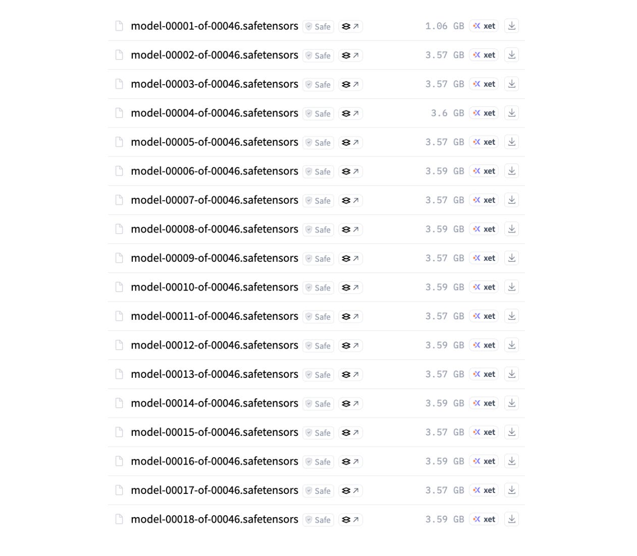
(Check out the config.json and model parameter files for the DeepSeek-V4-Flash model to understand this better.)
A model loader uses this file to build the model skeleton and then loads the parameters into the CPU memory (also called System memory). This memory is typically Dynamic random-access memory (DRAM), which offers larger capacity and is cheaper than the GPU memory.
The model parameters are next transferred to the GPU's HBM (High Bandwidth Memory), also known as global memory (or, generally, VRAM). This transfer takes place over PCIe, a high-speed connection between the CPU and GPU.
Seen tensor.to('cuda') method while training models? This is what happens under the hood when you call this method.
HBM is a specialized type of DRAM designed for massive parallel data throughput. While CPU memory has a throughput of 50 to a few hundred GB/s, HBM can deliver a throughput of a few TB/s. Although fast, HBM is smaller and much more expensive than CPU memory.

What if the LLM is too big for the GPU memory?
Let’s go back to the config.json file for DeepSeek-V4-Flash, which is a Mixture-of-Experts model with 284 billion total parameters.
If each parameter of this model is loaded in FP8 (8-bit floating-point) precision, which means that 1 parameter is represented in 8 bits or 1 byte, the total memory requirement of this model for parameter storage will be:
284B parameters × 1 byte/ parameter = 284 GB
But this is not the only thing that the GPU HBM needs to store. We also need space for KV cache, activations, and other overheads.
The popularly used NVIDIA H100 GPU comes with 80 GB of HBM. This is nowhere near enough to store 284 GB of parameters, let alone the KV cache and others. This means that the parameters must be distributed across multiple GPUs.
A standard architecture for hosting a model is an 8-GPU NVIDIA HGX H100 server. This server has 8 H100 GPUs, each with 80 GB of HBM, which sums to a total of 640 GB of memory.
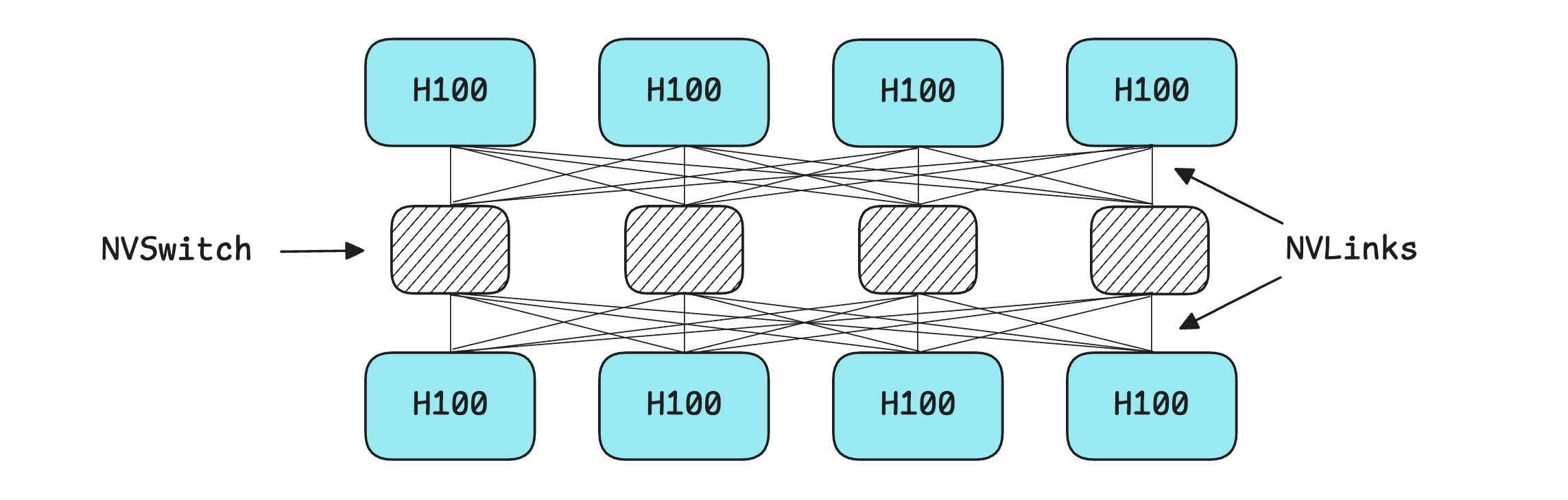
The GPUs in the server are linked using an NVSwitch, which provides each GPU with a full-bandwidth path to every other GPU, enabling them to transfer data fast enough (900GB/s) to behave as a single large accelerator.
The term “full-bandwidth” is important here because if no NVSwitch is used with NVLinks, the bandwidth is split between GPU pairs. In our 8-GPU setup, any single GPU-to-GPU pair would get only about 128 GB/s of bandwidth, compared to 900 GB/s (full bandwidth) with NVSwitch.
There are many techniques that are used to distribute the inference load across these GPUs. Some techniques split the model itself, while others split the input workload.
These are described as follows:
Tensor parallelism (TP): Splitting parameter/ weight matrices across GPUs, with each GPU performing part of the matrix multiplication and then syncing the results.
Pipeline parallelism (PP): Dividing the model’s layers across GPUs, with each GPU handling a consecutive block of layers and passing the activations to the next.
Context parallelism (CP): Splitting a single sequence and its KV cache across GPUs, with each GPU managing a part of the context to support very long sequence lengths.
Expert parallelism (EP): Distributing the experts of a Mixture-of-Experts (MoE) model across GPUs and routing the tokens to the GPU that holds their chosen experts.
Data parallelism (DP): Replicating the entire model on each GPU when it is small enough to fit, or replicating a fully sharded model across multiple GPU groups when the model is too large for a single GPU. Each replica then handles different user requests.
Hybrid parallelism: Combining several of these techniques discussed above. For example, TP, PP, CP, and EP are combined to create a complete sharded model replica. DP is then added by creating multiple such replicas, each serving different user requests in parallel.
If you’re completely new to these techniques, the following lesson will help.

What's next after loading parameters into GPU memory?
Once the parameters are loaded into GPU HBM, they are ready to process incoming user requests.
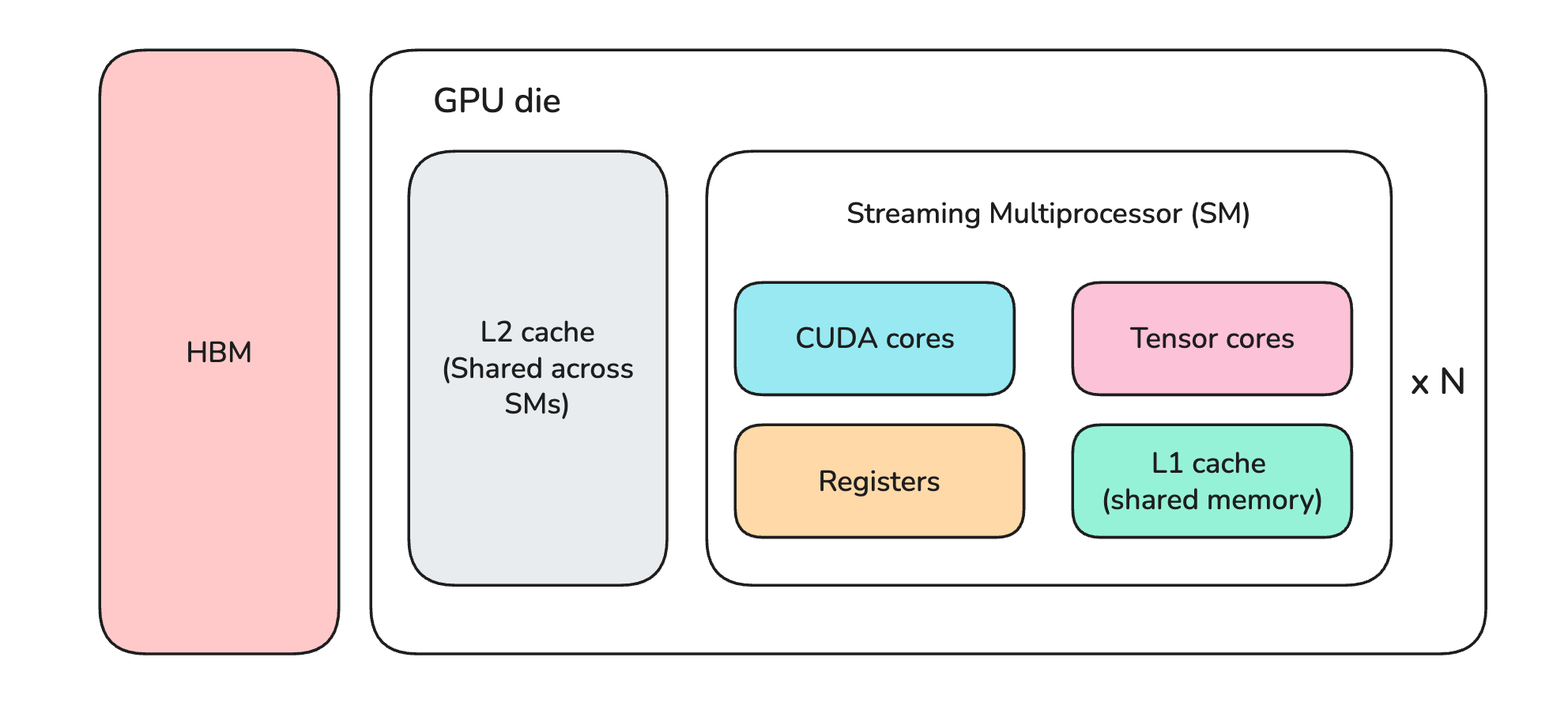
Let’s talk a bit about the main components of a GPU like the H100. These are:
Streaming Multiprocessors (SMs)
High-bandwidth memory (HBM)
On-chip memory
Streaming Multiprocessors, or SMs, are the processing units where calculations happen in a GPU. They contain thousands of smaller components called:
CUDA cores: that perform fast general mathematical operations
Tensor cores: that perform fast matrix operations (matrix multiplications)
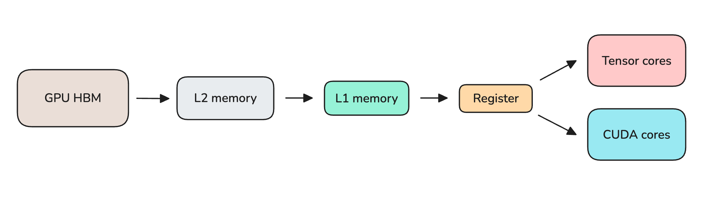
The on-chip memory is etched directly on the GPU die, unlike HBM, which is mounted alongside the die. This memory further consists of (arranged in ascending order of speed and descending order of capacity):
L2 memory/cache
L1 or shared memory/cache (shared across components of an SM)
Registers
On-chip memory components are Static random-access memory (SRAM), which is extremely fast but much smaller than other types of DRAM (CPU memory and GPU HBM) we discussed earlier.
For every user request/prompt, the model performs forward passes through its parameters in two phases: Prefill and Decode.
In each forward pass, every layer’s parameters are streamed from HBM to on-chip memory and then to the CUDA/Tensor cores, where the calculations actually occur. The weights are discarded once a token is produced, and this process repeats until the full sequence is generated or the maximum token-generation limit is reached.
If you want to better understand what calculations occur at the Transformer level, we have covered this in the previous lessons that you can find here:


What is Prefill and Decode?
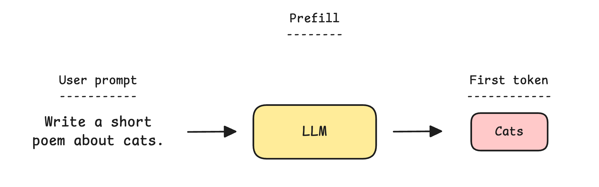
Prefill is the first phase where all tokens in a user’s prompt are processed together in a single forward pass through the LLM.
During this phase, each token computes a key (K) and value (V) vector, which are cached to build a KV cache for the entire initial user prompt. This KV cache is stored alongside the model parameters and intermediate activations in the HBM.
Prefill relies heavily on the GPU's tensor cores and is compute-bound. This is because all tokens of the initial user prompt are being processed in parallel.
A faster prefill means a shorter Time to First Token (TTFT), which is the delay before the model begins responding to the user's prompt.
Next comes Decode, the second phase, where the LLM generates one token at a time, with a single forward pass through the model for each token.
Instead of recomputing the key (K) and value (V) vectors for every previous token at each step, the model reuses these from the KV cache and only computes them for the new token. The newly computed K and V values are added to the KV cache for use in the next step of Decode.
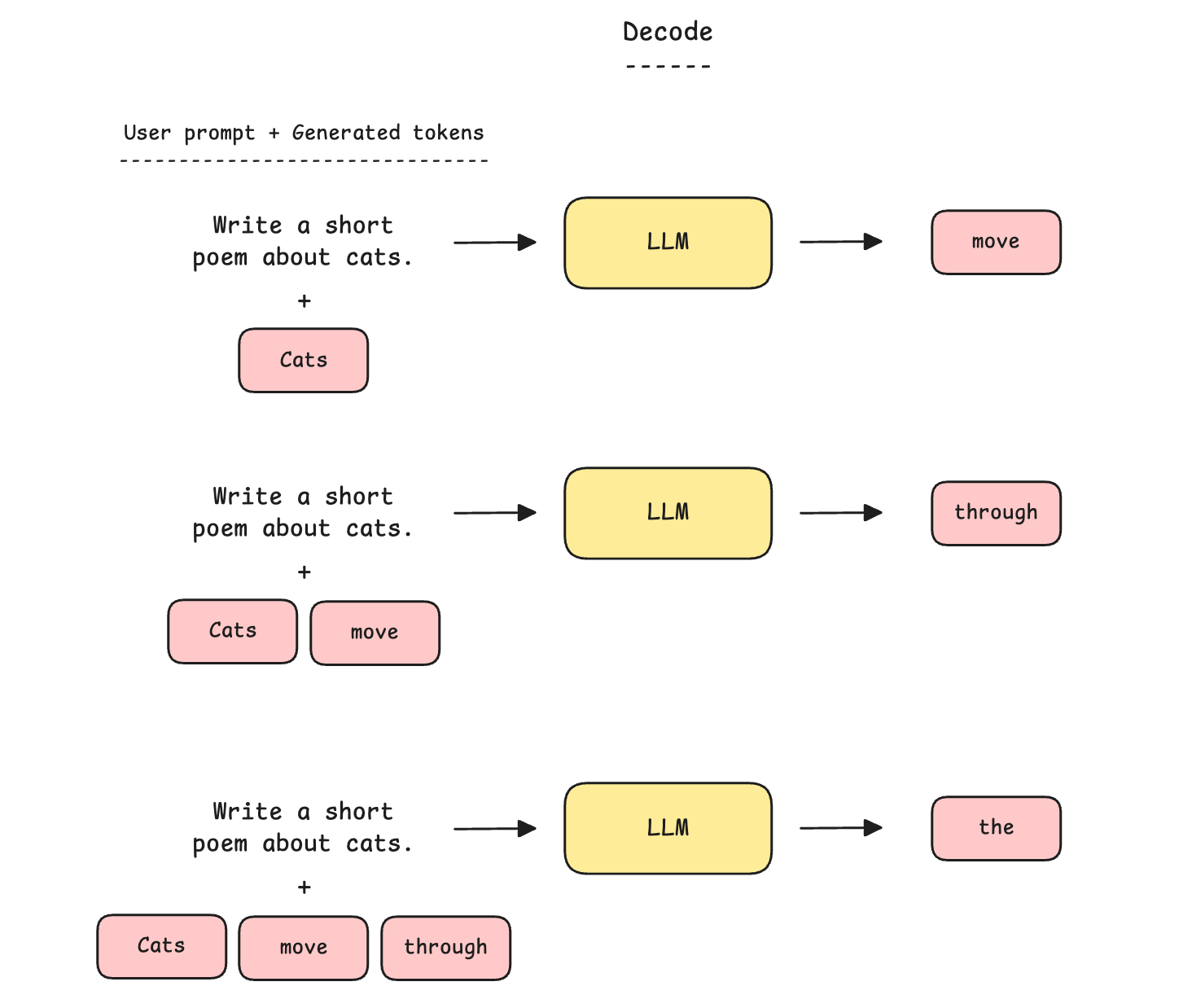
Decode is memory-bound and does not utilize the full capacity of the GPU’s Tensor cores. This is because, for every generated token, all model parameters must be streamed from HBM to the Tensor cores for a small amount of computation, discarded when the token is generated, and then re-read in full for the next token.
In this process, the calculations performed per token relative to the volume of weights moved are so small that the cores spend most of their time waiting on memory rather than computing.
Why is Decode memory-bound?
Let’s understand this better using an example.
Let’s say that we are using a 30B Dense model in 16-bit precision on a single H100 (with 80 GB of HBM). This is 60 GB of parameters (30B × 2 bytes).
To produce one token, all 60 GB are streamed from HBM to the Tensor cores. At the higher end of the H100’s memory bandwidth of 3.35 TB/s, it takes about 18 ms to generate one token. This gives a throughput of around 56 tokens per second.
Now let’s compare this with the computation involved.
A forward pass costs roughly 2 FLOPs per parameter per token (one multiply and one add operation), so the computational cost of processing a token through a 30B dense model is 60 GFLOPs (2 FLOPs × 30B).
The H100's Tensor cores can perform 990 TFLOP/s of FP16 operations. This means that 60 GFLOPs of operations will take around 0.06 ms (60 / 990,000).
Taken together, the computation takes roughly 0.06 ms, while streaming the 60 GB of weights takes 18 ms.
The cores only compute for 0.3% of the time required for the memory transfer. For the rest, they sit idle, waiting for the next set of parameters to arrive, making Decode memory-bound.
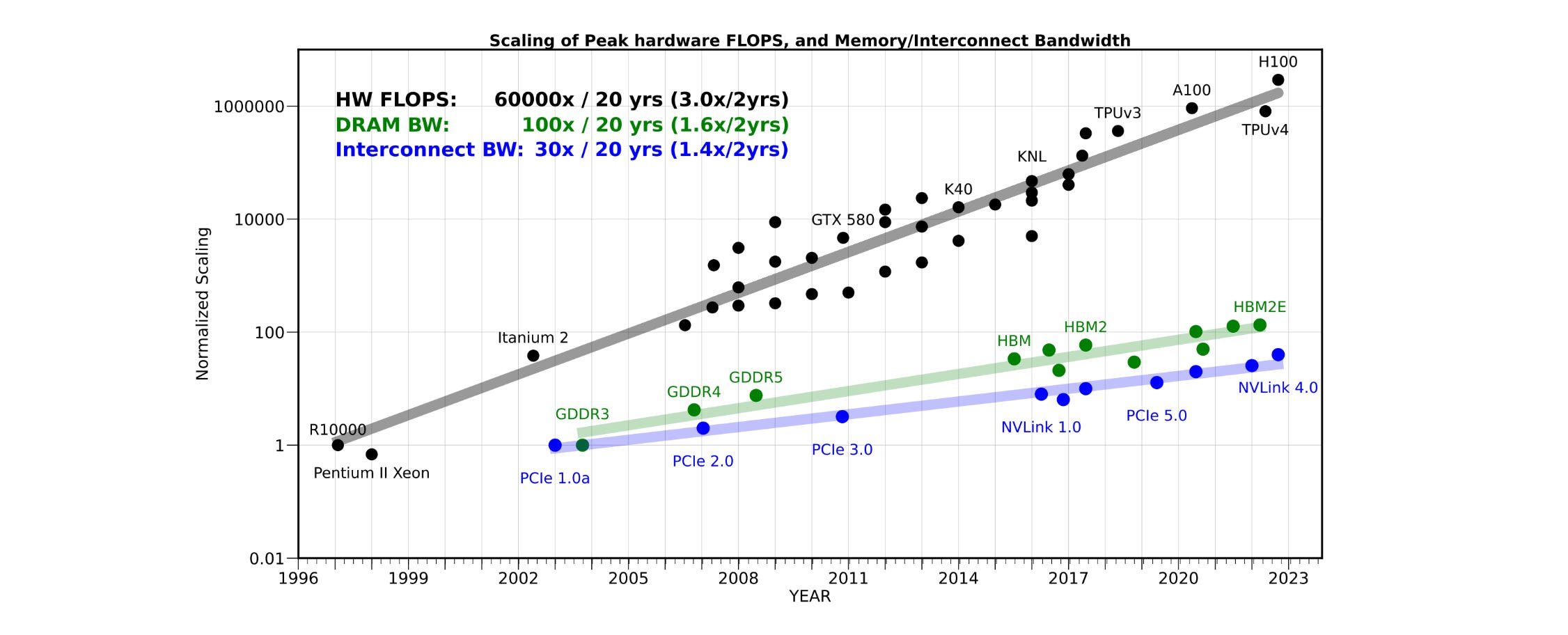
Over the past 20 years, peak server hardware FLOPS has scaled by a factor of 3 every 2 years, outpacing the growth of DRAM and interconnect bandwidth, which have scaled by factors of 1.6× and 1.4× every 2 years, respectively. This has made memory (and not compute) the primary bottleneck in LLM inference. (Source)
Why is the KV Cache so important for Decode?
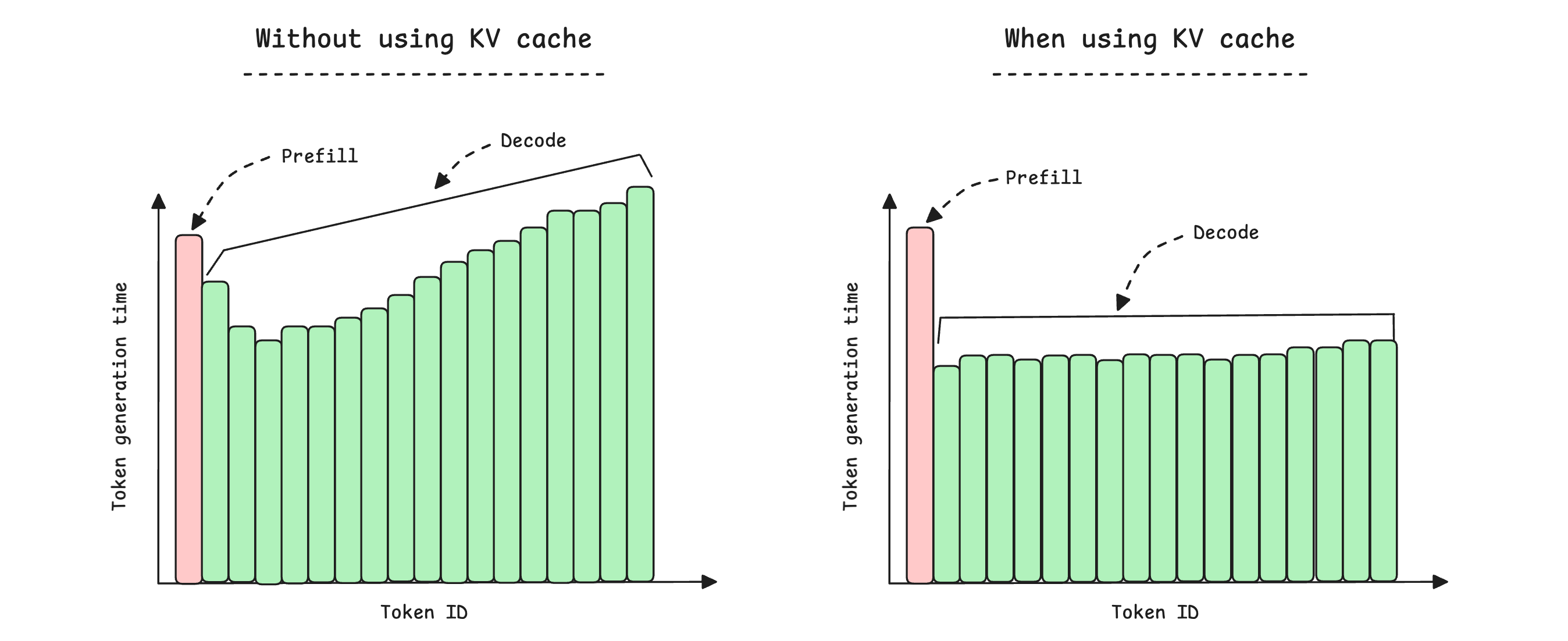
The KV cache ensures that the keys (K) and values (V) for past tokens are computed once and stored, so each Decode step computes only one new token's K and V and reads the rest from cache.
This slows the increase in the cost of generating a single token as the sequence length grows, making Decode faster and more efficient.
You must remember that using a KV cache is not always a “free lunch” since it also takes space in the HBM. As its size grows (with increasing context length and the number of batched requests), it could consume as much memory as the parameters themselves. Managing its size is something that one needs to keep in mind when serving LLMs.
TL;DR
To summarise:
During inference, model parameters are moved from SSD to CPU memory, GPU HBM, on-chip memory, and finally to the computation cores.
Models that are too large for a single GPU are split across multiple GPUs using multiple parallelism techniques.
The multi-GPU server uses NVSwitch to connect the GPUs, resulting in full communication bandwidth between them.
Each inference request is processed in two phases: Prefill and Decode.
Prefill processes all prompt tokens at once. It is a compute-bound process, and the Time to First Token (TTFT) depends on it.
Decode generates one token at a time. It is memory-bound and acts as the bottleneck of inference. This is because each token generation involves moving a large number of parameters while performing very little computation, leaving the GPU's computation cores mostly idle while waiting on memory.
The KV cache helps keep token generation costs from growing rapidly as sequence length increases.
KV cache also consumes HBM alongside model parameters and must be managed for efficient LLM serving.
✨ Courtesy of Backplanes, this newsletter edition is completely free to read. ✨
Show your love by liking it, restacking it, and sharing it with others! ❤️