
Build GPT in plain Python
Implement the GPT architecture in pure Python without using deep learning frameworks or dependencies

Andrej Karpathy recently published MicroGPT on GitHub. This is an elegant implementation of GPT in pure Python, and a gold mine for curious AI engineers.
In this article, we will dissect this code step by step and learn as much as possible from it.
Let’s begin!
Join the paid tier today to get access to all posts on this newsletter:
and so many more!
1. Python standard library imports
The implementation imports the Python standard libraries but skips any AI-related libraries, such as numpy or torch.
import os              # Interface to the operating system
import math            # For math calculations
import random          # For pseudo-random number generation
import urllib.request  # For downloading files from the internet

random.seed(42)        # Set the seed for reproducible results
2. Loading the dataset
A simple text file of names is used as the training database. A portion of it looks as follows.
This file is available here and loaded as follows.
# If the dataset file does not exist locally
if not os.path.exists('input.txt'):

    # The URL to the dataset
    names_url = 'https://raw.githubusercontent.com/karpathy/makemore/988aa59/names.txt'

    # Download it and save it locally as 'input.txt'
    urllib.request.urlretrieve(names_url, 'input.txt')

# Open the file and read it line by line
# .strip() removes whitespace
# "if line.strip()" skips empty lines
docs = [line.strip() for line in open('input.txt') if line.strip()]

# Shuffle the names list in the file and make its ordering random
random.shuffle(docs)

# Print how many names are there in the file (dataset)
print(f"Num docs: {len(docs)}")

# Num docs: 32033
This gives 32,033 names or training samples for the GPT model to learn from.
3. Setting up the Tokenizer
The Tokenizer maps each unique character (token) in the dataset to a unique number (its token ID).
It then adds one extra special token called BOS (Beginning of sequence) that is used to mark the start and end of a name (training sample/ sequence).
In bigger GPT models, one uses a separate EOS (End of sequence) token for marking the end of a sequence. Karpathy uses a simplified approach here, using just one token (BOS) to mark both the start and the end of the sequence.
The Vocabulary of the model is the total number of distinct tokens it knows.
The Vocabulary size is the number of unique characters in the dataset plus one (for the BOS token).
# 1. Join all names into one big string
# 2. Turn it into a set to get the unique characters
# 3. Sort them
# Each character's position in the resulting list becomes its token id (0, 1, 2, ..., 25).
uchars = sorted(set(''.join(docs)))

# Print the characters
print(uchars)
# ['a', 'b' ... 'z']

# The BOS token is assigned a token ID of 26
BOS = len(uchars)

# Vocabulary size is number of unique characters + 1 (for the BOS token)
vocab_size = len(uchars) + 1

# Print the vocabulary size
print(f"Vocab size: {vocab_size}")
# Vocab size: 27
4. Building a simple Automatic Differentiation engine
Autograd is the automatic differentiation engine used in PyTorch.
During the forward pass of neural network training, it records the differentiable operations performed on the inputs and parameters, and builds a graph of how the final loss was computed.
During the backward pass, it walks the graph in reverse and uses the chain rule to compute the gradient of the loss with respect to each parameter. These gradients tell us how much each parameter contributed to the error.
An optimizer then uses them to tweak the parameters in the direction that lowers the loss.
Since no dependencies are being used, Karpathy builds a simpler version of Autograd, based on his previous implementation, Micrograd, that works on numbers (scalars) rather than tensors.
In this differentiation engine, each Value wraps a number/ scalar and remembers how it was computed (which other Values it came from and the local derivative with respect to each).
Every math operation on a Value returns a new Value that records this information and builds up a computation graph.
During the backward pass, the graph is topologically sorted and traversed in reverse order from the output node, applying the chain rule to compute the derivative of the output (loss) with respect to each node in the graph.
# Differentiation engine

class Value:
    # __slots__ tells Python which instance attributes this class has.
    # This saves memory and speeds up attribute access.
    __slots__ = ('data', 'grad', '_children', '_local_grads')

    def __init__(self, data, children=(), local_grads=()):
        self.data = data                 # Scalar value of this node calculated during forward pass
        self.grad = 0                    # Derivative of the loss w.r.t. this node calculated in backward pass
        self._children = children        # Children of this node in the computation graph
        self._local_grads = local_grads  # Derivative of this node w.r.t. each child

    # Math operations on Values
    # Each operation also records its local derivative, used later in the backward pass.

    # Addition:  c = a + b
    def __add__(self, other):
        other = other if isinstance(other, Value) else Value(other)
        return Value(self.data + other.data, (self, other), (1, 1))

    # Multiplication:  c = a * b
    def __mul__(self, other):
        other = other if isinstance(other, Value) else Value(other)
        return Value(self.data * other.data, (self, other), (other.data, self.data))

    # Power:  c = a ** n
    def __pow__(self, other): return Value(self.data**other, (self,), (other * self.data**(other-1),))

    # Natural log:  c = log(a)
    def log(self): return Value(math.log(self.data), (self,), (1/self.data,))

    # Exponential:  c = exp(a)
    def exp(self): return Value(math.exp(self.data), (self,), (math.exp(self.data),))

    # ReLU:  c = max(0, a)
    def relu(self): return Value(max(0, self.data), (self,), (float(self.data > 0),))

    # Negation:  c = -a   (implemented as a * -1)
    def __neg__(self): return self * -1

    # Subtraction:  c = a - b   (implemented as a + (-b))
    def __sub__(self, other): return self + (-other)

    # Division:  c = a / b   (implemented as a * b^(-1))
    def __truediv__(self, other): return self * other**-1

    # Right-handed operators
    # These make expressions like  2 + a,  2 - a, 2 * a,  2 / a  work,
    # where a number is on the left side of a Value
    def __radd__(self, other): return self + other          # For 2 + a
    def __rsub__(self, other): return other + (-self)       # For 2 - a
    def __rmul__(self, other): return self * other          # For 2 * a
    def __rtruediv__(self, other): return other * self**-1  # For 2 / a

    # Backward pass to compute the gradient of this node w.r.t. every
    # ancestor in the computation graph
    def backward(self):
        # Topological sort all nodes in the graph (children before parents)
        # to process them in reverse
        topo = []
        visited = set()
        def build_topo(v):
            if v not in visited:
                visited.add(v)
                for child in v._children:
                    build_topo(child)
                topo.append(v)
        build_topo(self)

        # The gradient of the final output w.r.t. itself is 1 (the starting point)
        self.grad = 1

        # Navigate the graph in reverse and apply the chain rule where
        # each node passes its gradient down to its children multiplied
        # by the local derivative (dparent/dchild)
        for v in reversed(topo):
            for child, local_grad in zip(v._children, v._local_grads):
                child.grad += local_grad * v.grad
5. Defining Hyperparameters & Parameters
The GPT model's hyperparameters are defined as follows.
# Model hyperparameters

n_layer = 1      # Number of transformer layers (Depth of the model)
n_embd = 16      # Size of each token's vector (Width of the model)
block_size = 16  # Maximum context length the model can attend over (The longest name is 15 chars)
n_head = 4       # No. of attention heads
head_dim = n_embd // n_head  # Dimension of each attention head
These are used to build randomly initialized matrices with weights for the following, where every weight is a Value so that the differentiation engine can track it.
Token embeddings
Position embeddings
Each layer's attention head
2-layer MLP
Final output head
# Helper function to make a (n_out x n_in) shaped matrix of Values, initialized with small random numbers
matrix = lambda n_out, n_in, std=0.08: [[Value(random.gauss(0, std)) for _ in range(n_in)] for _ in range(n_out)]

# Dictionary holding all the model's weight matrices
state_dict = {
    'wte': matrix(vocab_size, n_embd),     # Token embeddings
    'wpe': matrix(block_size, n_embd),     # Position embeddings
    'lm_head': matrix(vocab_size, n_embd), # Final output head
}

# Add per-layer weights for each transformer block
for i in range(n_layer):
    state_dict[f'layer{i}.attn_wq'] = matrix(n_embd, n_embd)      # Query projection in Attention head
    state_dict[f'layer{i}.attn_wk'] = matrix(n_embd, n_embd)      # Key projection in Attention head
    state_dict[f'layer{i}.attn_wv'] = matrix(n_embd, n_embd)      # Value projection in Attention head
    state_dict[f'layer{i}.attn_wo'] = matrix(n_embd, n_embd)      # Output projection in Attention head
    state_dict[f'layer{i}.mlp_fc1'] = matrix(4 * n_embd, n_embd)  # Up-projection in the MLP
    state_dict[f'layer{i}.mlp_fc2'] = matrix(n_embd, 4 * n_embd)  # Down-projection in the MLP
Going back to the architecture of a Decoder-only Transformer will help if you do not understand this step well.

Finally, all of the weights are flattened into one params list for the optimizer to update later.
# Flatten every weight into a single list so the optimizer can loop over them
params = [p for mat in state_dict.values() for row in mat for p in row]

print(f"No. of model params: {len(params)}")
# No. of model params: 4192
6. Defining helper functions for building the model
The following three are defined next:
linear: a fully-connected layer with no bias termsoftmax: to convert a list of logits into a probability distributionrmsnorm: to normalize a vector by its root-mean-square for regularization
# Fully connected layer with no bias term
def linear(x, w):
    # For each output row 'w_row' in weight matrix 'w',take the dot product with input vector 'x'
    return [sum(w_i * x_i for w_i, x_i in zip(w_row, x)) for w_row in w]

# Softmax function
def softmax(logits):
    # Max logit
    max_val = max(val.data for val in logits)

    # Subtract the max logit before exponentiating to prevent overflow
    exps = [(val - max_val).exp() for val in logits]

    # Normalize the exponentials so that they sum to 1
    total = sum(exps)
    return [e / total for e in exps]

# RMS Norm
def rmsnorm(x):
    # Compute the mean of the squared values
    mean_sq = sum(x_i * x_i for x_i in x) / len(x)

    # Define scale factor = 1 / sqrt(mean square)
    # 1e-5 prevents divide-by-zero error
    scale = (mean_sq + 1e-5) ** -0.5

    # Rescale every element so the vector has unit root-mean-square
    return [x_i * scale for x_i in x]
7. Building the model and its forward pass
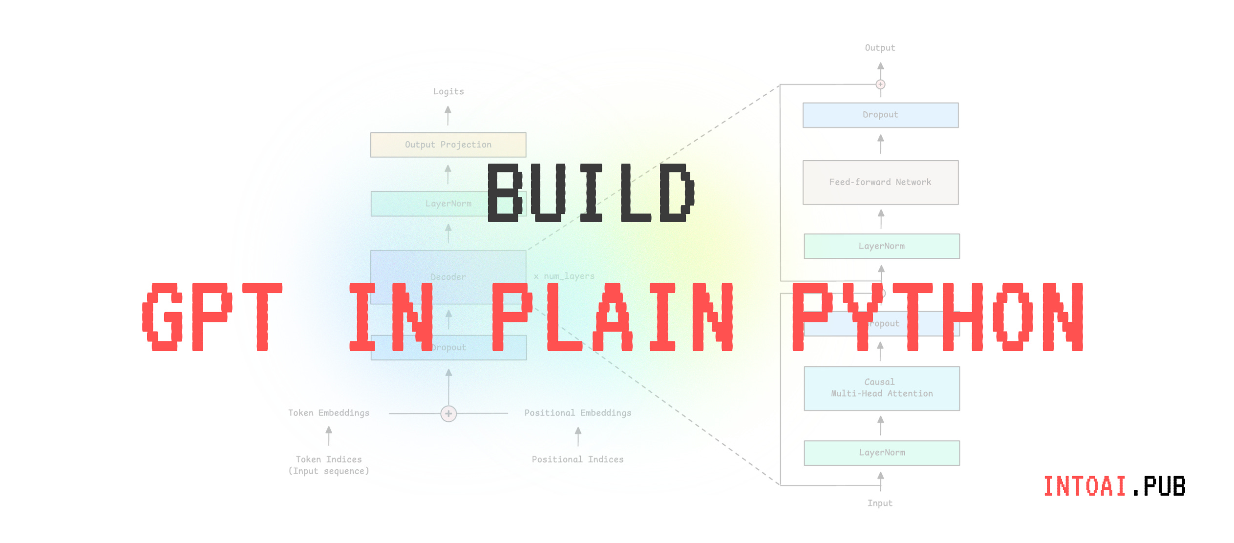
Karpathy builds a GPT-2 style model but with three minor architectural differences:
RMSNorm is used instead of LayerNorm
No bias terms are used
ReLU activation is used instead of GeLU
During the forward pass of a single token through this model, its token and position embeddings are looked up, summed, and run through n_layer transformer blocks.
Each transformer block consists of two sub-blocks, each implementing RMSNorm and residual connections. These are:
Multi-head causal self-attention
2-layer MLP with ReLU
After the final transformer block, an output head produces vocabulary logits for predicting the next token.
For faster inference, the model uses a KV cache to store each transformer block’s past keys (K) and values (V), so it only computes new K and V for the current token instead of recomputing them for all previous ones.
# GPT forward pass for a single token
def gpt(token_id, pos_id, keys, values):
    tok_emb = state_dict['wte'][token_id]           # Look up token's embedding vectors
    pos_emb = state_dict['wpe'][pos_id]             # Look up token's position embedding
    x = [t + p for t, p in zip(tok_emb, pos_emb)]   # Sum up the embeddings
    x = rmsnorm(x)                                  # Initial RMSNorm

    for li in range(n_layer):
        # Multi-head self-attention block
        x_residual = x  # Save input for the residual connection
        x = rmsnorm(x)  # Pre-norm before attention

        # Project the input into Query, Key, and Value vectors
        q = linear(x, state_dict[f'layer{li}.attn_wq'])
        k = linear(x, state_dict[f'layer{li}.attn_wk'])
        v = linear(x, state_dict[f'layer{li}.attn_wv'])

        # Append the new K, V to this layer's KV cache
        keys[li].append(k)
        values[li].append(v)

        x_attn = []

        for h in range(n_head):
            # Slice out this head's portion of Q, K, V
            hs = h * head_dim
            q_h = q[hs:hs + head_dim]
            k_h = [ki[hs:hs + head_dim] for ki in keys[li]]
            v_h = [vi[hs:hs + head_dim] for vi in values[li]]

            # Scaled dot-product attention scores between current Q and every cached K
            attn_logits = [
                sum(q_h[j] * k_h[t][j] for j in range(head_dim)) / head_dim ** 0.5
                for t in range(len(k_h))
            ]

            # Softmax over past timesteps to get attention weights
            attn_weights = softmax(attn_logits)

            # Weighted sum of value vectors (This is the attention head's output)
            head_out = [
                sum(attn_weights[t] * v_h[t][j] for t in range(len(v_h)))
                for j in range(head_dim)
            ]

            # Concatenate heads
            x_attn.extend(head_out)

        # Output projection
        x = linear(x_attn, state_dict[f'layer{li}.attn_wo'])

        # Residual connection
        x = [a + b for a, b in zip(x, x_residual)]

        # MLP block
        x_residual = x     # save input for the residual connection
        x = rmsnorm(x)     # Pre-norm before MLP
        x = linear(x, state_dict[f'layer{li}.mlp_fc1'])  # Up-projection
        x = [x_i.relu() for x_i in x]                    # ReLU activation
        x = linear(x, state_dict[f'layer{li}.mlp_fc2'])  # Down-projection
        x = [a + b for a, b in zip(x, x_residual)]       # Residual connection

    # Final projection from hidden state to vocabulary logits (output head)
    logits = linear(x, state_dict['lm_head'])

    return logits
8. Building the Optimizer
The Adam optimizer is set up next.
It keeps a running estimate of the gradient's first moment (mean, m) and second moment (uncentered variance, v) for every parameter, using exponential moving averages controlled by beta1 and beta2.
# Hyperparameters for the Adam optimizer
learning_rate, beta1, beta2, eps_adam = 0.01, 0.85, 0.99, 1e-8

# First and second moment estimates for each parameter
m = [0.0 for _ in params]  # First moment (mean of gradients)
v = [0.0 for _ in params]  # Second moment (variance of gradients)
9. Training the model
The training loop runs for 1000 steps.
Each step involves:
Pick one training sample (name) from the dataset
Converting it into character-level tokens
Adding BOS tokens on both sides of the sample
Next, the model processes the sample token by token, predicting the next token at each position. It then calculates cross-entropy loss using the predicted and true values, and averages the losses for each position into a single value for the entire name.
The loss.backward() method then goes through the computation graph in reverse and calculates how much each parameter contributed to the loss.
Finally, the Adam optimizer uses these gradients to adjust each parameter so that the loss is reduced the next time.
Note that this training loop is not optimized and will take many minutes to complete!
# Training loop

# Number of training steps
num_steps = 1000

for step in range(num_steps):
    # Pick the next training sequence and convert it into token ids, with BOS on each end
    doc = docs[step % len(docs)]
    tokens = [BOS] + [uchars.index(ch) for ch in doc] + [BOS]

    # Number of next-token predictions to make, capped at block_size
    n = min(block_size, len(tokens) - 1)

    # Empty KV caches for this sequence
    keys, values = [[] for _ in range(n_layer)], [[] for _ in range(n_layer)]
    losses = []

    # Go through each position in the sequence, predict the next token, measure the loss
    for pos_id in range(n):
        token_id, target_id = tokens[pos_id], tokens[pos_id + 1]

        # Forward pass to get next-token logits
        logits = gpt(token_id, pos_id, keys, values)

        # Convert logits to probabilities using softmax
        probs = softmax(logits)

        # Cross-entropy loss for this position
        loss_t = -probs[target_id].log()

        # Add to the 'losses' list
        losses.append(loss_t)

    # Average loss across all positions in the document
    loss = (1 / n) * sum(losses)

    # Backpropagation
    loss.backward()

    # Update each parameter using Adam with linear learning-rate decay over training
    lr_t = learning_rate * (1 - step / num_steps)

    for i, p in enumerate(params):
        # Update running estimates of the gradient's mean (m) and squared mean (v)
        m[i] = beta1 * m[i] + (1 - beta1) * p.grad
        v[i] = beta2 * v[i] + (1 - beta2) * p.grad ** 2

        # Bias-correct the moment estimates
        m_hat = m[i] / (1 - beta1 ** (step + 1))
        v_hat = v[i] / (1 - beta2 ** (step + 1))

        # Adam parameter update
        p.data -= lr_t * m_hat / (v_hat ** 0.5 + eps_adam)

        # Zero the gradient for the next step
        p.grad = 0

    # Print progress
    print(f"step {step+1:4d} / {num_steps:4d} | loss {loss.data:.4f}", end='\r')
10. Generating text from the model
Once the model is trained, we use it to produce new names.
Text generation starts with the BOS token and empty KV caches.
At each step, the model predicts the next token’s logits, which are divided by a temperature value before applying softmax. This converts the logits into probabilities, which are used to select the next token.
The temperature value controls how creative the model output is. A lower value makes the model produce more common outputs, while a higher value makes it produce more unusual and creative outputs.
The generated token is fed back into the model to again produce the next token, building the name one character at a time.
Text generation goes on till the model outputs a BOS token (signaling the end of a name) or when the maximum generation length is reached.
# Text generation/ Inference

temperature = 0.3  # Controls randomness/ creativity of outputs

print("--- Inference (New, hallucinated names) ---\n")
print(f"Temperature: {temperature}\n")

for sample_idx in range(20):
    # Start each sample fresh with empty KV caches and the BOS token
    keys, values = [[] for _ in range(n_layer)], [[] for _ in range(n_layer)]
    token_id = BOS

    sample = [] # This holds the characters of the name being generated

    # Generate one character at a time, up to block_size characters
    for pos_id in range(block_size):
        # Obtain logits for the next token
        logits = gpt(token_id, pos_id, keys, values)

        # Scale logits by temperature and convert to probabilities
        probs = softmax([l / temperature for l in logits])

        # Randomly choose a token based on these probabilities
        token_id = random.choices(range(vocab_size), weights=[p.data for p in probs])[0]

        # If the BOS token is generated, stop text generation
        if token_id == BOS:
            break

        # Look up the character for this token and add it to the name being generated
        sample.append(uchars[token_id])

    # Join all the characters together and print the generated name
    print(f"sample {sample_idx+1:2d}: {''.join(sample)}")
Here are the interesting names the model generates at temperature values of 0.3 and 1.5.
--- Inference (New, hallucinated names) ---

Temperature: 0.3

sample  1: kanaya
sample  2: jarila
sample  3: anisa
sample  4: arish
sample  5: arist
sample  6: karie
sample  7: kana
sample  8: anany
sample  9: aleten
sample 10: anla
sample 11: karion
sample 12: rara
sample 13: aria
sample 14: laran
sample 15: lara
sample 16: kara
sample 17: aran
sample 18: areni
sample 19: halia
sample 20: kare
--- Inference (New, hallucinated names) ---
Temperature: 1.5
sample 1: zabr
sample 2: upeqodm
sample 3: don
sample 4: maxnp
sample 5: numtyenaa
sample 6: brcti
sample 7: hica
sample 8: nanity
sample 9: iaushan
sample 10: rnays
sample 11: ketydanzf
sample 12: dlemainq
sample 13: zidoj
sample 14: gycsen
sample 15: xem
sample 16: yhiega
sample 17: larlinayn
sample 18: yjalsonma
sample 19: danfmayz
sample 20: beenSuper interesting!
Share this article with others and earn some referral rewards. ❤️
Join the paid tier today to get access to all posts on this newsletter:
and so many more!
You can also read my books on Gumroad and connect with me on LinkedIn to stay in touch.