


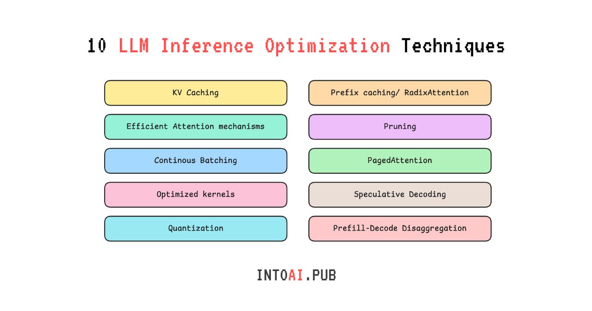
LLM inference optimization is one of the hottest topics today, and everyone wants text generation that's faster, more accurate, and cheaper. Here are 10 techniques that can help you get there.
1. KV Caching
During a step of autoregressive text generation, an LLM compares the last token’s Query vector to the Key vectors of all previous tokens, including itself. This creates attention weights, which are used to compute a weighted sum over the corresponding Value vectors. This results in the attention output for that token.
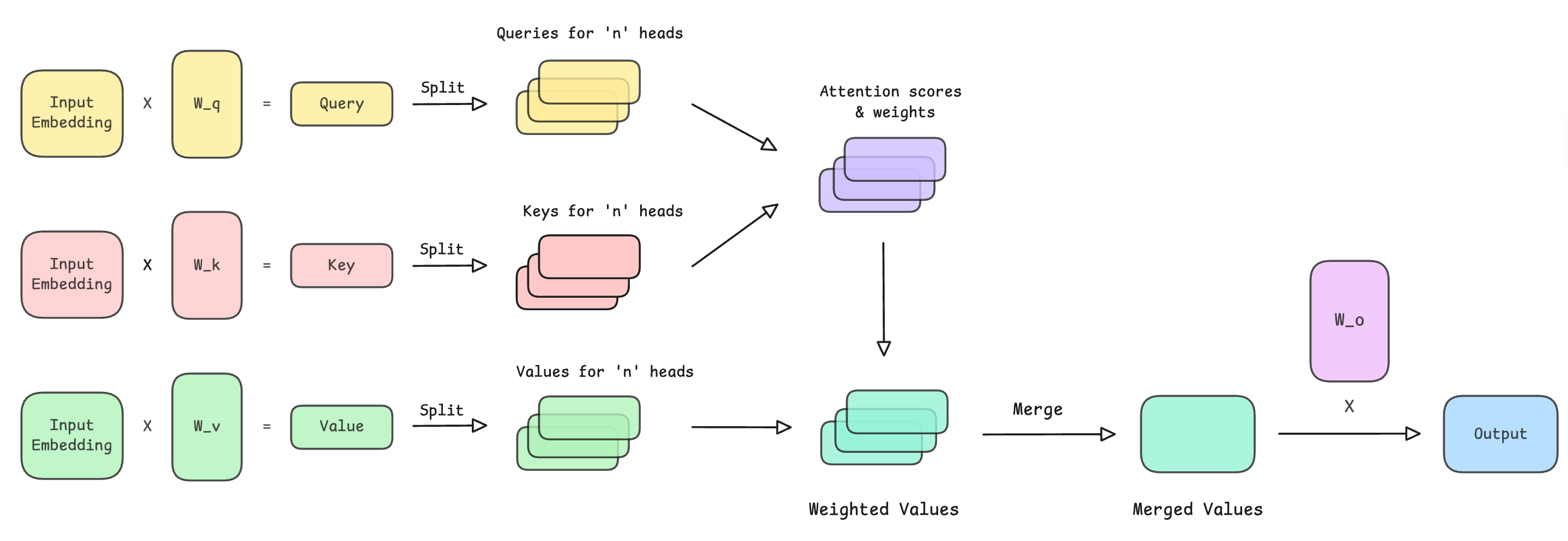
For example, considering a word as a token, when generating the token after "The capital of the U.K. is", the LLM:
Converts the current token ("is") into a Query vector
Scores it against the Key of each preceding token to find that "capital" and "U.K." are most related to it
Combines those tokens' Value vectors to decide that the next token is most likely to be "London"
This process is repeated at each step of text generation.
Calculating Key and Value vectors for all previous tokens at each step is expensive, especially as the sequence length grows. Using a KV cache helps solve this issue of repeated computations.
The KV cache stores each token’s Key and Value vectors once, rather than recomputing them for the entire sequence at each step. This means the LLM now has to calculate (and append to the KV cache) only the new token’s Key and Value, reusing the rest from the cache at each step.
This massively reduces the amount of computation during inference but comes at the cost of using up HBM memory. (There’s no free lunch!)
Using KV caching is one of the simplest techniques that you can take to improve inference.
Before we move forward, I want to introduce you to my book, ‘LLMs In 100 Images’.
It is a collection of 100 easy-to-follow visuals that describe the most important concepts you need to master to understand LLMs today.
I’m offering a limited-time 30% discount, which you can claim using the button below.
2. Efficient Attention mechanisms
As we discussed earlier, the KV cache takes space in a GPU’s HBM, and managing its size helps make inference fast.
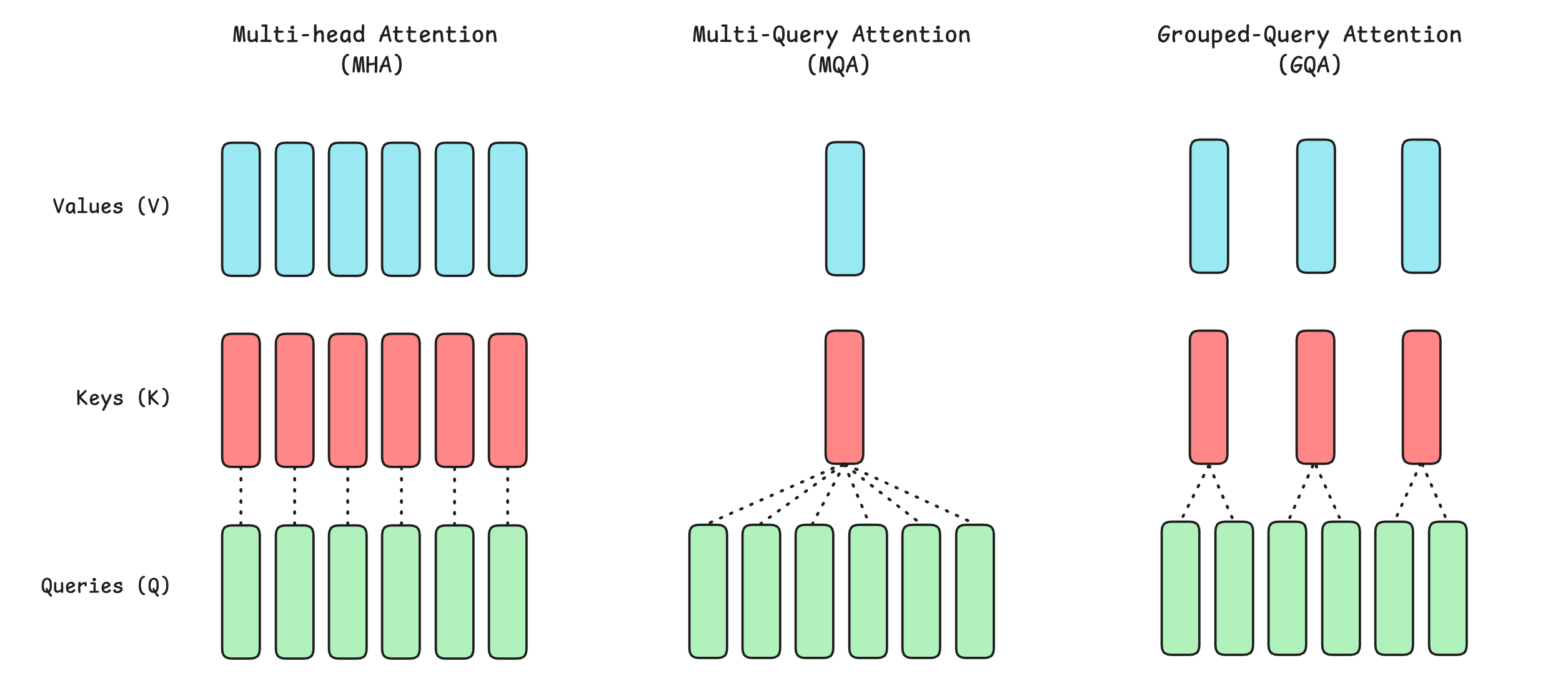
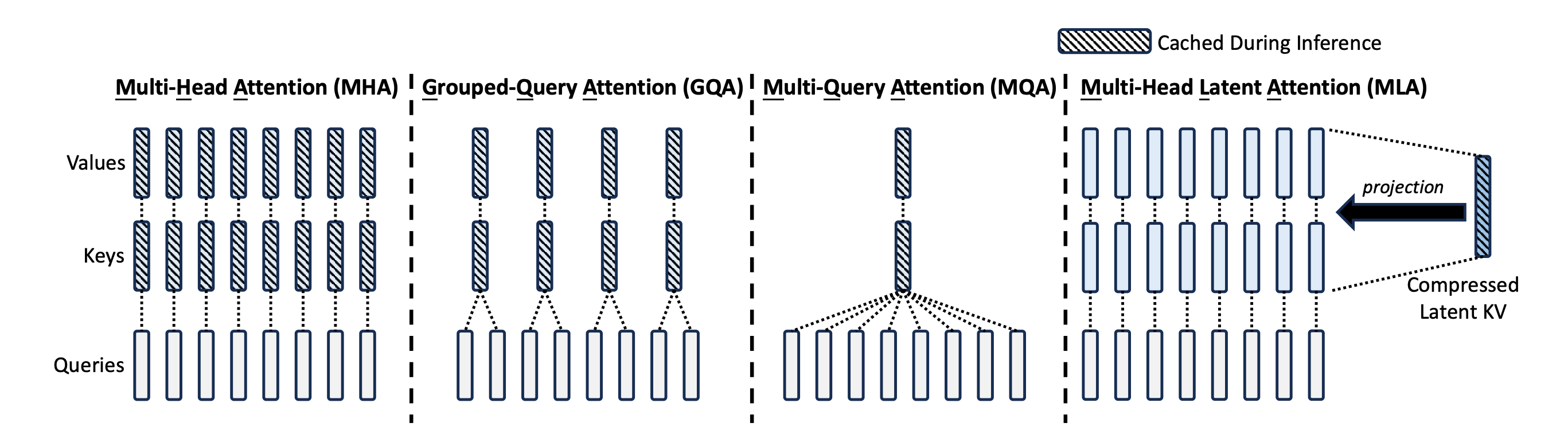
The traditional Multi-head self-attention (MHA) uses multiple heads, each with its own Key and Value vectors.
There are a few attention variants that reduce the number of Key and Value vectors used (and therefore the KV cache size) as follows:
In Multi-Query Attention (MQA), all attention heads share the same Key (K) and Value (V) vectors, while each head still has its own Query (Q) vector.
In Grouped Query Attention (GQA), Query (Q) heads are grouped, and each group shares one Key (K) and Value (V).
There is also Multi-head Latent Attention (MLA), which compresses the Key and Value vectors into a low-dimensional latent vector and caches it. This uses much less memory than the full-sized KV cache. The full Key and Value vectors are reconstructed from this latent vector when needed.
3. Continuous Batching
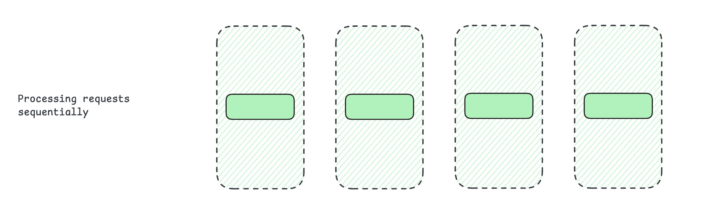
A naive way to process LLM requests is to handle them sequentially. This is very inefficient, as different requests can arrive at different times and can have variable input and output lengths (and therefore processing times).
Requests are therefore batched and processed together. This improves the system's overall throughput and reduces underutilized GPU compute.
Batching can be done at the request and token levels. When done at the request level, the system has to wait for a certain predetermined number of requests to arrive and be batched before they can be processed. This is called Static Batching.
A system can also be configured to wait only until a pre-decided maximum time rather than indefinitely to fill the full batch before the batch can start processing. This is called Dynamic Batching.
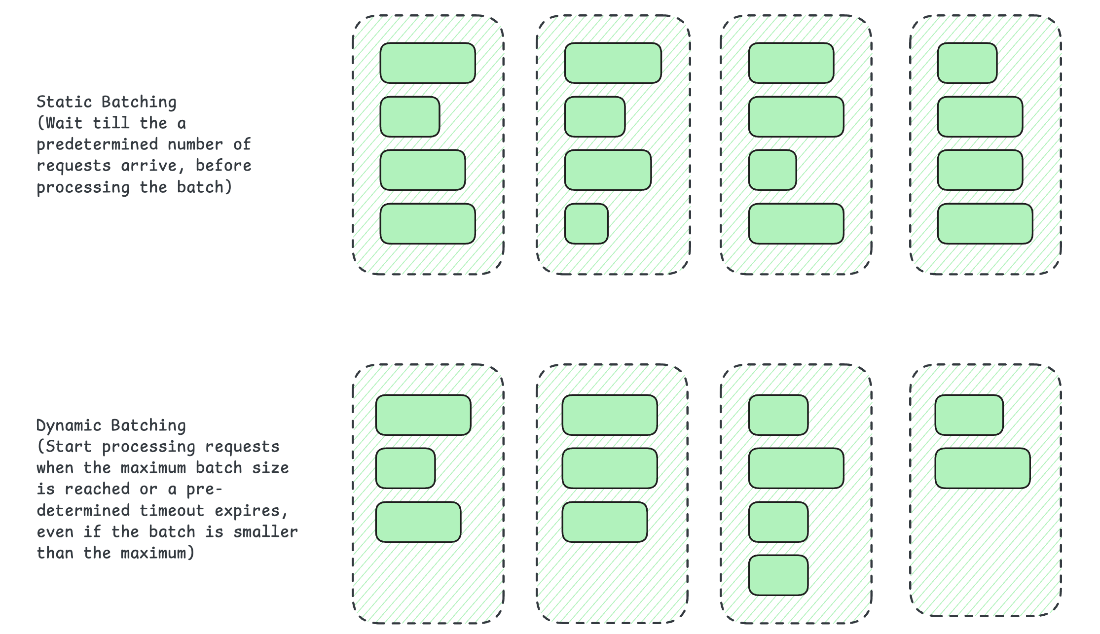
In either case, the entire batch must finish processing before any new request can join.
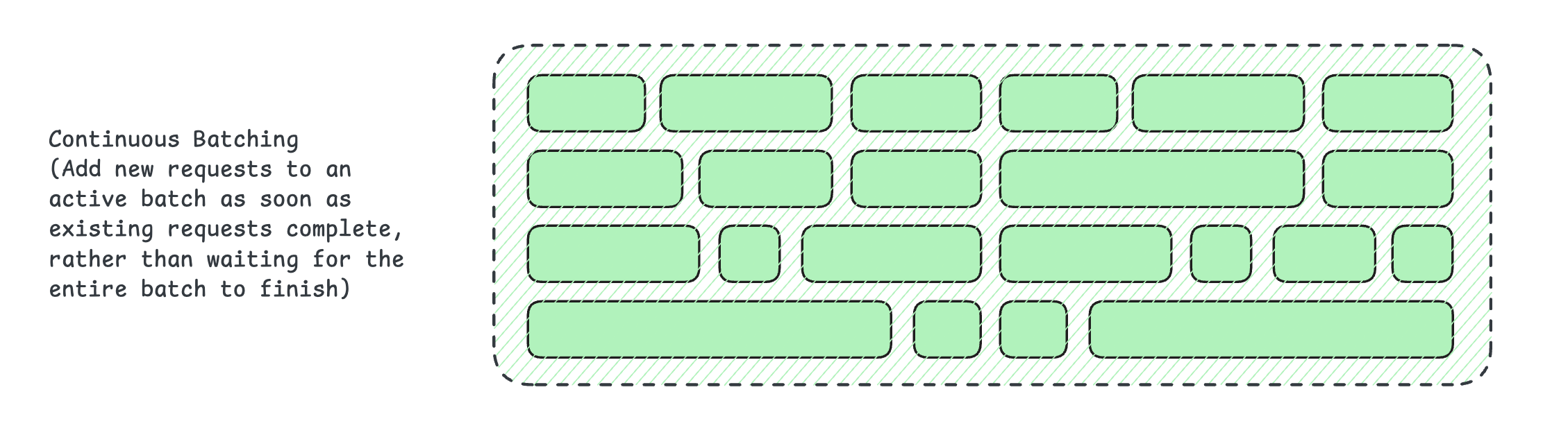
In contrast, when done at the token level, as in Continuous (in-flight) batching, requests are processed token by token. Instead of waiting for the entire batch to finish, the system evicts a completed request and immediately fills the vacated slot with a new request. This helps utilize GPU resources more effectively than the previous two approaches.
4. Optimized Kernels
Inference Decode is memory-bound, which means that the GPU spends more time moving data from memory (HBM) to the compute cores than performing computations.
A kernel is a function that runs on a GPU and performs multiple parallel operations. A kernel can be optimized to keep data in on-chip memory (SRAM/registers), avoid re-reading it from the slow HBM, and feed it to the compute cores to better use them.
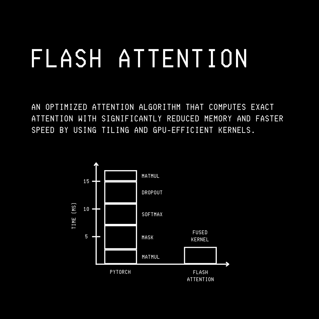
This can be done using Kernel fusion, a technique in which multiple individual operations in an algorithm are merged (“fused”) into a single kernel to avoid data movement across memory.
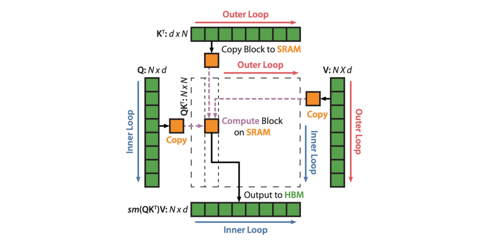
FlashAttention is a well-known example of this, in which operations from the attention computation are merged into a single kernel.
This is how standard attention is computed:
Query and Key matrices are read from HBM and multiplied to produce an attention score matrix in the compute cores
This matrix is written back to the HBM
The matrix is re-read to apply Softmax
The result is written back to the HBM
The result is read back to multiply it by the Values matrix to create the final output of attention computation, finally writing it back to the HBM
FlashAttention avoids all this data movement by never creating the full attention matrix in HBM. It splits the Query, Key, and Value matrices into smaller blocks called Tiles that fit in on-chip SRAM and performs attention calculations one tile at a time.
The attention scores and softmax are computed on-chip, and only the final output is written back to the HBM. This reduces data movement between HBM and the compute cores, resulting in faster attention calculations using far less memory.
5. Quantization
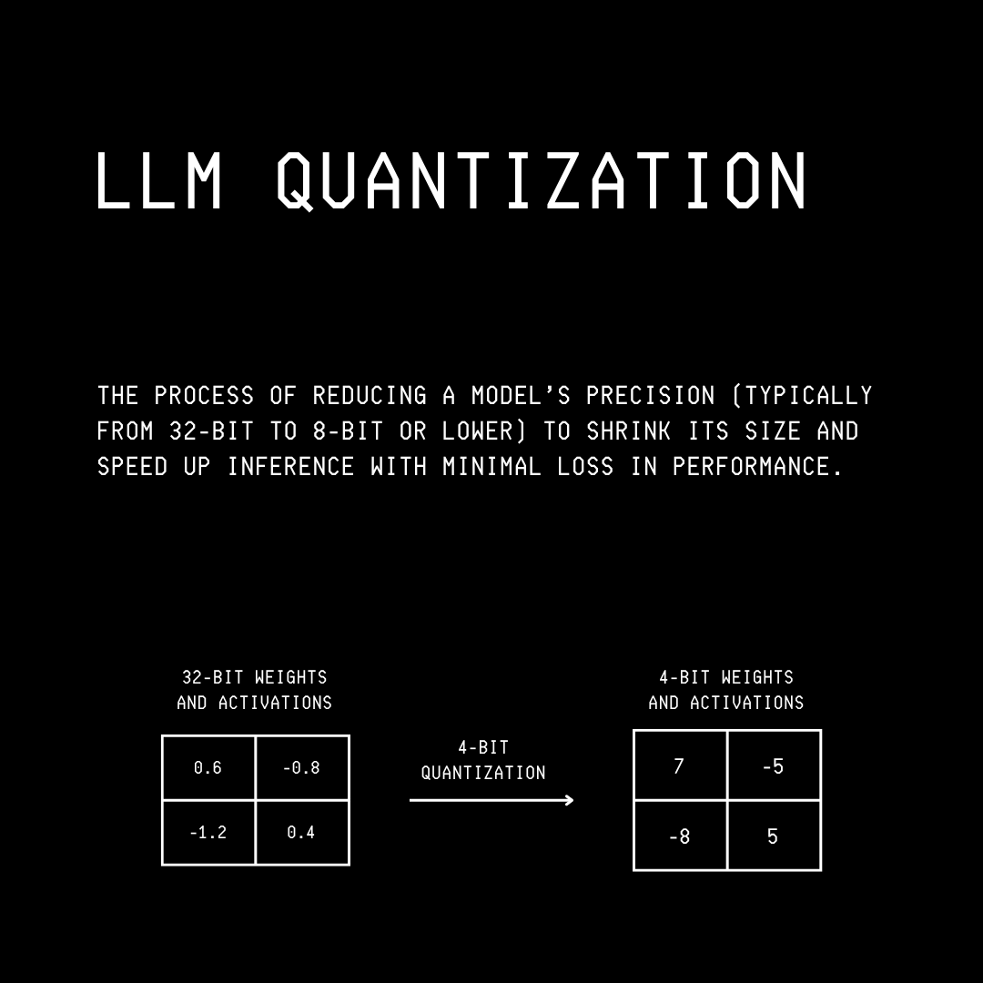
Quantization is the process of storing and computing LLM parameters, activations, and KV cache in lower-precision formats such as INT8 (8 bits) and INT4 (4 bits) instead of full-precision 32-bit floating-point (FP32) or 16-bit floating-point (FP16 or BF16) formats.
This reduces the model's memory requirements and increases inference throughput by reducing data transferred from HBM to the compute cores, at the cost of a slight drop in accuracy.
Take the example of Llama 3 70B. In full precision (FP32), each parameter occupies 4 bytes of memory. The total memory requirement for this model is 280 GB (70B parameters X 4 bytes/parameter). This means it will not fit on a single H100 GPU with only 80 GB of memory.
Reducing the precision to INT4, each parameter occupies 0.5 bytes of memory, and the total memory requirement for this model reduces to 35 GB (70B parameters × 0.5 bytes per parameter), making it possible to fit it on a single GPU.
A commonly used convention for quantized models is W(x)A(y) which tells how much a model’s weights (W) and activations (A) have been quantized. For example:
W4A16with 4-bit weights and 16-bit activationsW8A8with 8-bit weights and 8-bit activationsW4A4with 4-bit weights and 4-bit activations
You will also find quantized models suffixed with “-GPTQ” and “-AWQ”. These are the commonly used techniques for model quantization:
6. Prefix / Prompt caching & RadixAttention
LLM inference has two phases:
Prefill, where all tokens in the input prompt are processed together, making it compute-bound. Prefill determines the Time-to-first-token (TTFT), and it is when the KV cache is built.
Decode, where subsequent tokens are generated one at a time, making it memory-bound since very little computation is done at each step. Decode determines the Time per Output Token (TPOT).
Prefix (or prompt) caching is an optimization technique that reuses the computed KV cache for a shared portion/ prefix of the input prompt across multiple user requests. This reduces redundant computation during Prefill and leads to a shorter Time-to-first-token (TTFT).
For example, consider a long system prompt “System: You are a helpful assistant…”.
Without prefix caching, each user request computes Prefill for all tokens in the system prompt and the user's question.
With prefix caching, the KV cache for the system prompt is computed once and stored. Every user request then reuses it and computes Prefill only for the user's actual question.
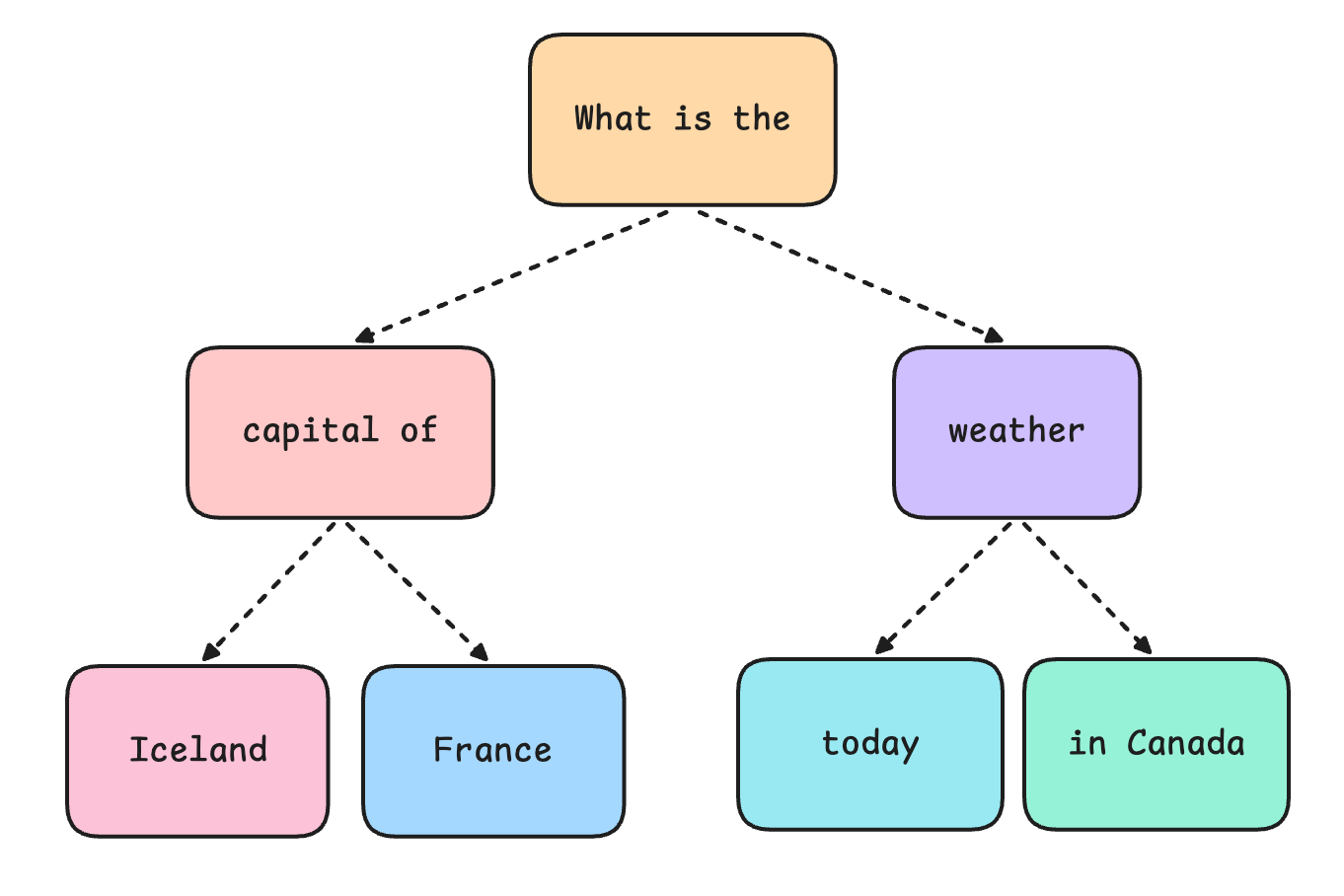
RadixAttention is a technique introduced with the SGLang serving framework that efficiently implements Prefix caching using a data structure called a radix tree.
In a radix tree, each path from the root is a token sequence, and shared prefixes (prompt portions common to user requests) are shared branches.
For a new user request, the algorithm walks the radix tree, matching tokens as far as possible and reusing the KV cache along the matched path. Prefill is computed only for the unique tokens in the user request.
7. Pruning
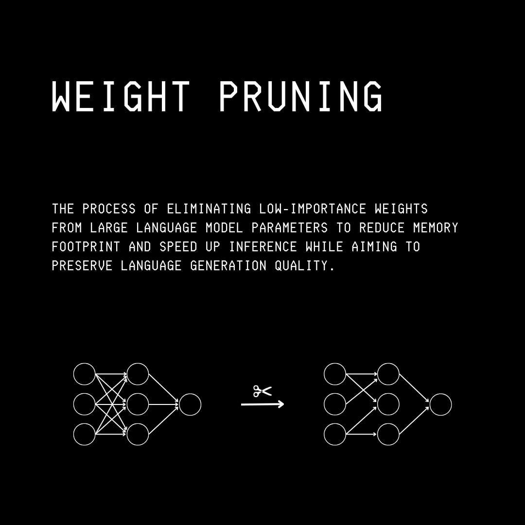
Pruning is the technique of removing parts of a model that do not contribute much to its accuracy, making it smaller and therefore cheaper to perform inference on.
Pruning can be done in three ways:
Unstructured pruning: Involves setting low-magnitude individual parameters to zero
Structured pruning: Involves removing complete sections (neurons, attention heads, fully-connected layers) of the model
Semi-structured (N: M) pruning/ sparsity: Involves setting
Nof everyMconsecutive weights to zero. Newer NVIDIA GPUs (Ampere onward) have hardware support for 2:4 sparsity, which leads to ~2x increase in matrix multiplication throughput.
8. PagedAttention
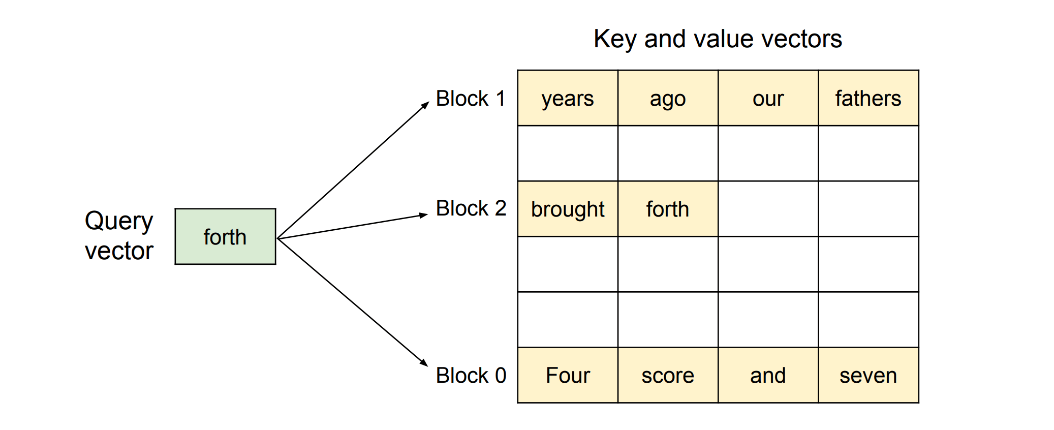
PagedAttention is a technique introduced in the vLLM serving framework to efficiently manage the KV cache's memory requirements. The technique is inspired by how operating systems manage memory using Paging.
Instead of storing the KV cache in a single large contiguous chunk of GPU memory upfront, it is dynamically stored in multiple fixed-size, small, non-contiguous blocks called pages.
A per-sequence block table maps logical token positions to physical memory blocks, and the attention kernel uses it to locate the correct KV pairs when needed.
9. Speculative Decoding
Speculative Decoding is a technique used to accelerate inference with large LLMs.
To do so, it uses a smaller LLM from the same family as the larger one, with both sharing the tokenizer and vocabulary. The smaller LLM in this case is called the ‘Draft model’, and the larger LLM is called the ‘Target model‘. This smaller LLM naturally runs inference faster because it has fewer parameters than the larger one.
This is how it works:
For a given prompt, the smaller/ Draft model first generates
Ktokens (a draft). This is the Speculation/ Drafting step.
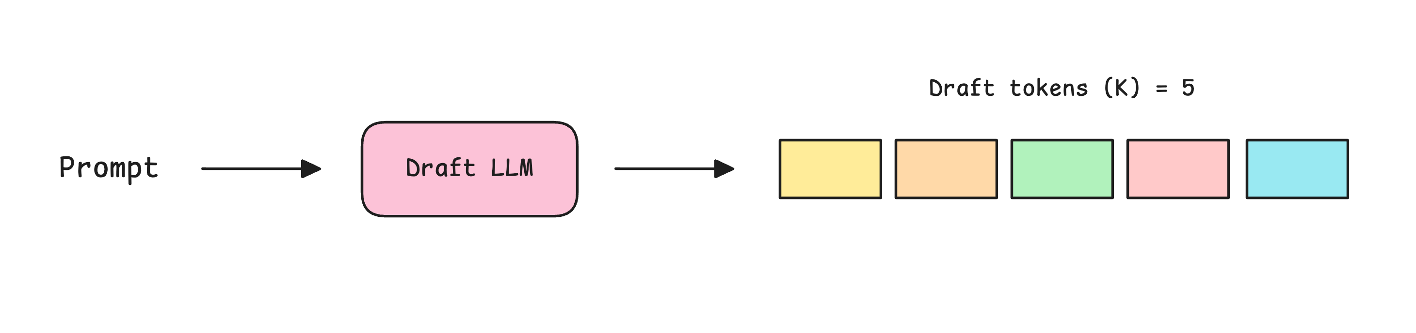
These
Ktokens, along with the original prompt, are given to the larger/ Target model.
In a single forward pass, the larger model outputs its probability distribution for the next token at every position in the draft, plus one for an additional position beyond it. So the total number of target predictions isK + 1 = 6. Because Decode is memory-bound, this single forward pass takes almost as long as generating just one token from the model.

Next comes the Verification step. Each drafted token is checked against the larger/ target model’s prediction at that position. If they agree (when using greedy decoding) or the target finds it likely enough (when using probabilistic decoding via rejection sampling), the token is accepted.
At the first token where this check fails, that token and all subsequent drafted tokens are discarded, and the larger model provides a replacement token for that position. All subsequent tokens from the target LLM are also discarded because they were conditioned on the rejected drafted token.
Drafting then resumes from this position.
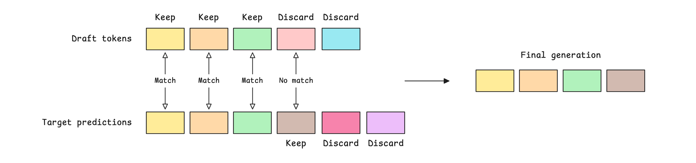
The benefits from this are quite evident.
Consider a case where all
Kdraft tokens are accepted, we getK+1tokens in the final output. This is the best-case scenario.More commonly, if the first
idraft tokens are accepted, we geti+1tokens, i.e.idraft tokens + 1 resampled replacement token from the target model.In the worst case, if the first draft token is rejected, we get just 1 token, which is the resampled replacement token from the target model. This is the same as normal decoding from the target model.
If you want to read more about Speculative Decoding, please check out the following lesson.

10. Prefill-Decode Disaggregation
We have previously discussed that:
Prefill is compute-bound and determines the Time to first token (TTFT)
Decode is memory-bound and determines the Time Per Output Token (TPOT), also called Inter-token latency (ITL)
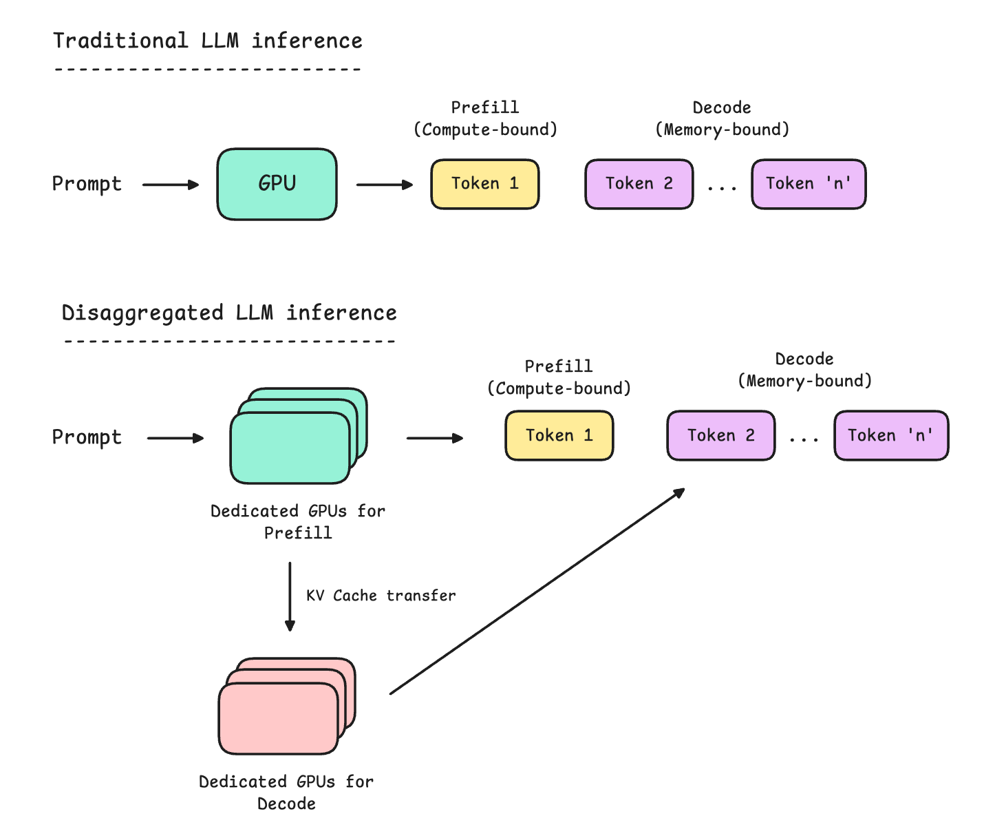
These are two fundamentally different problems, and optimizing each on a single GPU can be tough, especially when the prompts are long relative to the outputs (prefill-heavy requests), and one wants both low TTFT and TPOT at the same time.
Prefill-decode disaggregation is a serving architecture that helps in this case by moving the two stages of inference to separate dedicated pools of GPUs.
In this case, the dedicated pool of GPUs for Prefill would be optimized for higher compute, while the dedicated pool of GPUs for Decode would be optimized for higher memory bandwidth and capacity.
For example, the H200 GPU, compared to the H100, has much faster and larger memory but the same core compute. Therefore, H200s are best used in the Decode pool, and H100s in the Prefill pool.
One of the major overheads in this serving technique is transferring the KV cache between the Prefill-dedicated GPU pool and the Decode-dedicated GPU pool, which can be optimized with faster interconnects such as NVLink or InfiniBand.
Thanks for reading this article. If you found it valuable, show your love by liking it, restacking it, and sharing it with others! ❤️
Join the paid tier today to get access to all posts in this newsletter, including:
and so many more!