
A Deep Dive Into Universal Reasoning Models
A deep dive into what Universal Reasoning Models (URMs) are, how they work and what makes them achieve groundbreaking results on the ARC-AGI benchmarks with such a simple architecture.

Recursive reasoning models are a promising architectural candidate that could lead us towards AGI.
One of the earliest recursive reasoning models, called the Hierarchical Reasoning Model (HRM), was introduced by Sapient Intelligence in early 2025.
This model surprised the AI community, as it achieved amazing results on complex benchmarks such as ARC-AGI, beating powerful LLMs with just 27 million parameters and training on only 1,000 examples.
Its architecture was further improved by a researcher at Samsung SAIT AI Lab. This new recursive reasoning model, called the Tiny Recursive Model (TRM), used a single small network with only two layers (a total of 7 million parameters) and achieved even better performance than the HRM.
We are moving very fast in this field, and a new recursive reasoning model called the Universal Reasoning Model has recently been introduced by researchers at Ubiquant.
This model further improves reasoning performance, surpassing both HRM and TRM, and achieving state-of-the-art 53.8% pass@1 on ARC-AGI 1 and 16.0% pass@1 on ARC-AGI 2.
What makes Recursive reasoning models perform so well is the recurrent inductive bias inherent in their foundational architecture, called the Universal Transformer.
Let’s talk about the Universal Transformer in depth next.
Thanks for reading Into AI! If you want to get even more value from this publication and support me in writing these in-depth articles, consider becoming a paid subscriber today.
Get access to posts like the following and more!


What Is A Universal Transformer?
Universal Transformer (UT) was introduced in a 2019 research paper that aimed to improve the early Transformer architecture by drawing inspiration from RNNs.
Transformers at the time failed to generalize to many simple tasks that RNNs handled with ease. This included copying strings or performing simple logical inference when the string/ formula lengths exceeded those observed at training time.
Researchers believed that the recurrent inductive bias of RNNs was what made them perform so well.
UTs were therefore built to combine the best of both worlds:
Parallelizability and better learning abilities (each token can attend to all other tokens’ states via Self-attention) of Transformers
Recurrent inductive bias of RNNs
How Does A Universal Transformer Work?
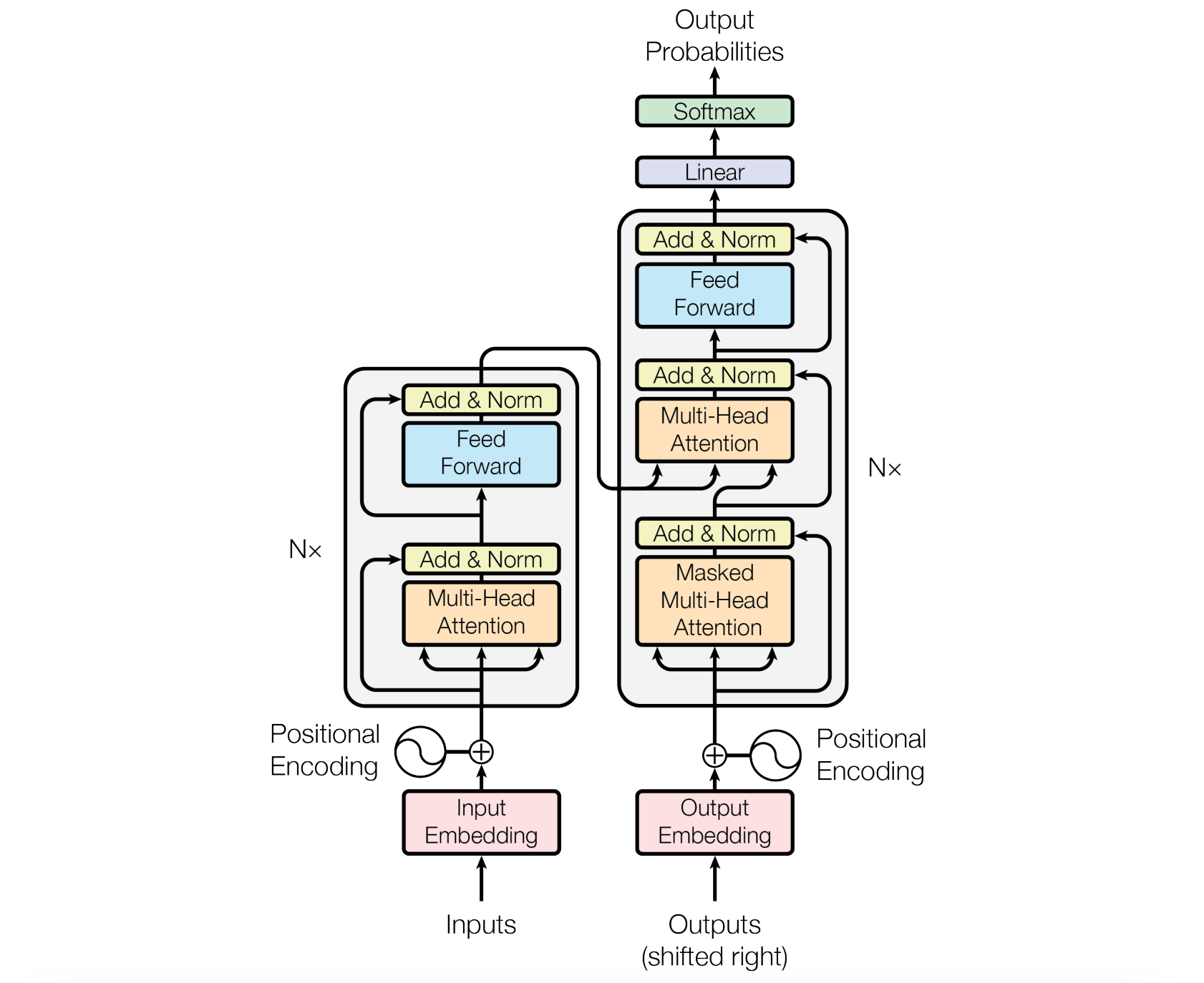
The Universal Transformer architecture is an encoder-decoder architecture just like the original Transformer.
This is how the encoder processes its inputs:
Given an input sequence to the encoder, it is converted into token embeddings, and positional and time-step encodings are added to the embeddings at every refinement step
Multi-head self-attention (MHA) is then applied to the token representation
After MHA, each token representation is passed through a Transition function, which is either a small feedforward network or a convolution. This transforms each token locally, as in an Feed-forward network (FFN) in a conventional Transformer.
Residual connections, dropout, and layer normalization are applied to stabilize training.
The refinement proceeds for T steps, reusing the same parameters at each step, and finally producing the encoder output.
The decoder shares the same basic recurrent architecture as the encoder, except it uses Causal or Masked self-attention, so each position can only attend to earlier positions (and not the future positions) in the output sequence.
The decoder also attends to the encoder’s final output (using Cross-attention labelled ‘Multihead Attention’ in the following image) so that each output token can be conditioned on the input sequence. In this case, the queries (Q) are generated from the decoder representations, and the keys and values (K and V) are generated from the encoder representations.
Just as the encoder, the decoder repeatedly refines its representations with shared parameters.
After the final step, the decoder’s output is projected to vocabulary logits and passed through a softmax to produce output probabilities.
Just like the conventional Transformer, the Universal Transformer is autoregressive and trained with Teacher forcing, where the decoder receives the target sequence shifted right during training.
During inference, the encoder runs only once, and the decoder generates tokens one at a time, each time conditioning on previously generated tokens and producing a probability distribution over the vocabulary via a final linear layer and softmax.
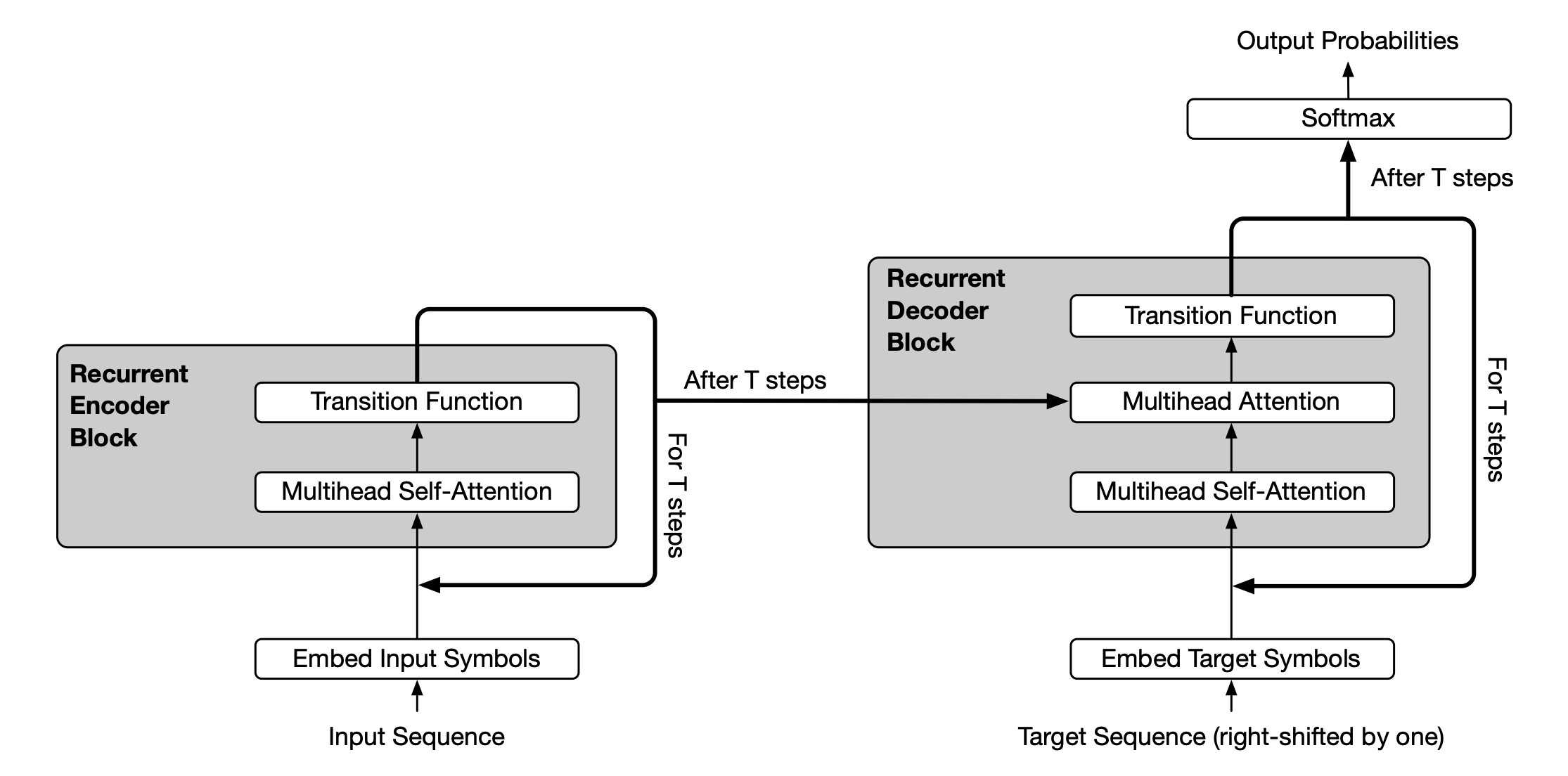
Compare this to the conventional encoder-decoder Transformer architecture as shown below.
Learning The Differences
UT vs RNN
An RNN processes tokens one at a time, passing information forward through the sequence (a token’s state depends only on the previous token’s hidden state).
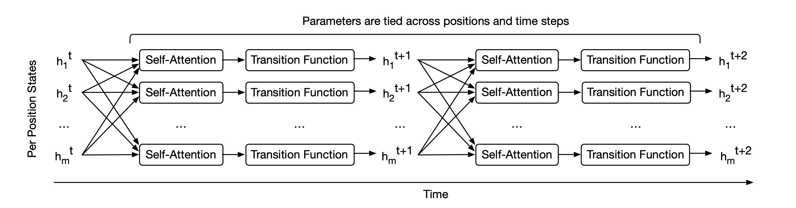
A UT, instead, updates all tokens in parallel at each step, and recurrence occurs over refinement steps rather than over sequence positions.
Universal Transformers can be thought of as applying self-attentive RNNs in parallel to all positions in the sequence.
UT vs Transformer
A standard Transformer iteratively processes its input by passing it through a fixed stack of layers with different weights.
On the contrary, a UT iteratively refines its representations by repeatedly applying a single Transformer block with shared weights.
Let’s understand this in more depth mathematically.
In a conventional Transformer, for an input token sequence x of length N coming from a vocabulary V is shown as:

A token embedding function ϕ, shown below, maps this sequence to one where each token has a d-dimensional embedding.

These initial embeddings are represented by H(0).

Next, a Transformer layer/ block, parameterized by θ, as shown below:

Composed of the following:
Feed-forward (FFN) network
Residual connections
LayerNorm (LN)
Is applied to the embeddings as follows.

where:

After processing through L Transformer layers, an unembedding function ψ, as shown below, projects the embedding back to the vocabulary logit space.

The complete conventional Transformer model M(std) of depth L is constructed by stacking L Transformer layers, each with its own parameters Θ = {θ(1),…, θ(L)}.

M(std) where the operator ◦ denotes function compositionIn this architecture, to achieve better reasoning performance, we generally need to increase its depth by adding more layers. But adding more layers comes with a rising number of parameters, and therefore a greater need for training and inference compute.
Universal Transformers take a different approach than this. Instead of stacking up L different layers, the UT applies a single Transformer block repeatedly to refine token representations.
Given an input token sequence x converted into token embeddings represented by H(t) at time step t, positional and time-step encodings are added to them at every refinement step.
Then, the MHA block is first applied as shown below.

Then, a position-wise Transition function, which is either a Feed-forward network (FFN) or a convolution, is applied as follows:

All attention and transition parameters denoted by Θ(UT) are reused for all time steps.

Unlike a fixed-layer Transformer, with a UT, it is possible to dynamically control the number of computation steps during inference and therefore model deeper algorithmic behaviors than a traditional Transformer.
Avoiding Wasted Computation With ACT
So far, we discussed that a UT runs a Transformer block for a fixed number of time steps, and each token is refined over those time steps.
But think about this: There are tokens that are easier to learn (e.g., common stop words) than other tokens that are harder to learn (e.g., tokens that track long-range dependencies or are used to make logical pivots).
So the natural question is whether we really need the same number of time steps to learn both, or whether we can determine how many refinement steps each token actually needs to be learned and save on wasted compute.
This is where ACT or Adaptive Computation Time comes in. This algorithm was introduced popularly in RNNs in a 2016 paper by Alex Graves, and goes as follows.
At each timestep t and each token position i, a halting probability is predicted:

where:
h(t, i)is the hidden state of the tokeniat timesteptwandbare learned parameters (Tis the transpose operation)σ is the sigmoid function that produces a value in the range 0 to 1
Each token keeps a running total of these probabilities as follows:

This goes on until:

where ϵ is a small constant.
The final token representation is a weighted mixture as follows:

where:
h(final)(i)is the final hidden state of a token at positionibefore unembedding to logitsΔ(t,i)called Truncated allocation, is a differentiable weight derived from the halting probabilities used so that the weighted sum of intermediate hidden states is equal to 1
Now that we understand the UT well (both recurrent computation and ACT), let’s move forward to understand how it leads to the Universal Reasoning Model (URM).
Building The Universal Reasoning Model
The Universal Reasoning Model (URM) is built on the base architecture of the Universal Transformer (UT) with the following three differences:
It uses the Decoder-only design with multiple Transformer layers (instead of the Encoder-Decoder design of the UT)
It uses the ConvSwiGLU module
It uses the Truncated Backpropagation Through Loops (TBPTL) algorithm
Let’s learn about ConvSwiGLU and TBPTL in more detail.
1. ConvSwiGLU
Before we understand how ConvSwiGLU works, we must understand what GLU and SwiGLU are.
We have previously learned about the Feed-forward network (FFN) in the Transformer architecture, whose role is to learn token-wise (rather than inter-token) patterns well by:
Processing each token independently of the others
Expanding dimensionality of token embeddings to increase representational capacity
Adding non-linearity to inputs using activation functions like GELU/ ReLU
Projecting them back to the original embedding dimension before passing them to the next layer
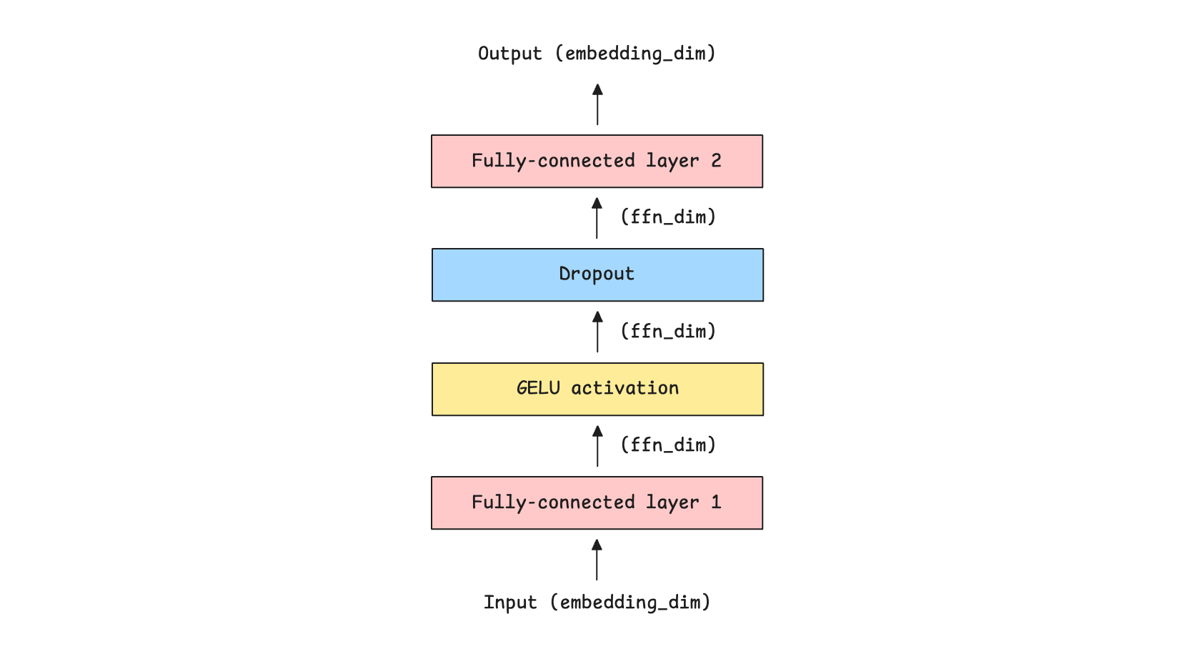
Mathematically, given an input X, the FFN applies two linear projections and an activation function where:
W(up)expands the dimensions (shown as Fully-connected layer 1 in the above)W(down)reduces them to the original dimension (shown as Fully-connected layer 2 in the above image)σ is an activation function, such as Sigmoid, GELU, or ReLU

Gated Linear Unit (GLU) takes this one step further by introducing gating, similar to that in LSTMs.
Instead of computing the following:

These two projections are computed:

The GLU operation is computed as follows, where ⊙ represents elementwise multiplications and σ is the Sigmoid activation function:

The final output from here is computed by applying W(down) as follows:

SwiGLU or Swish-Gated Linear Unit, simply replaces the sigmoid gate with the Swish/ SiLU activation function in GLU, as follows:

where:

and σ is the Sigmoid activation function.
The final output from here is again computed by applying W(down) as follows:

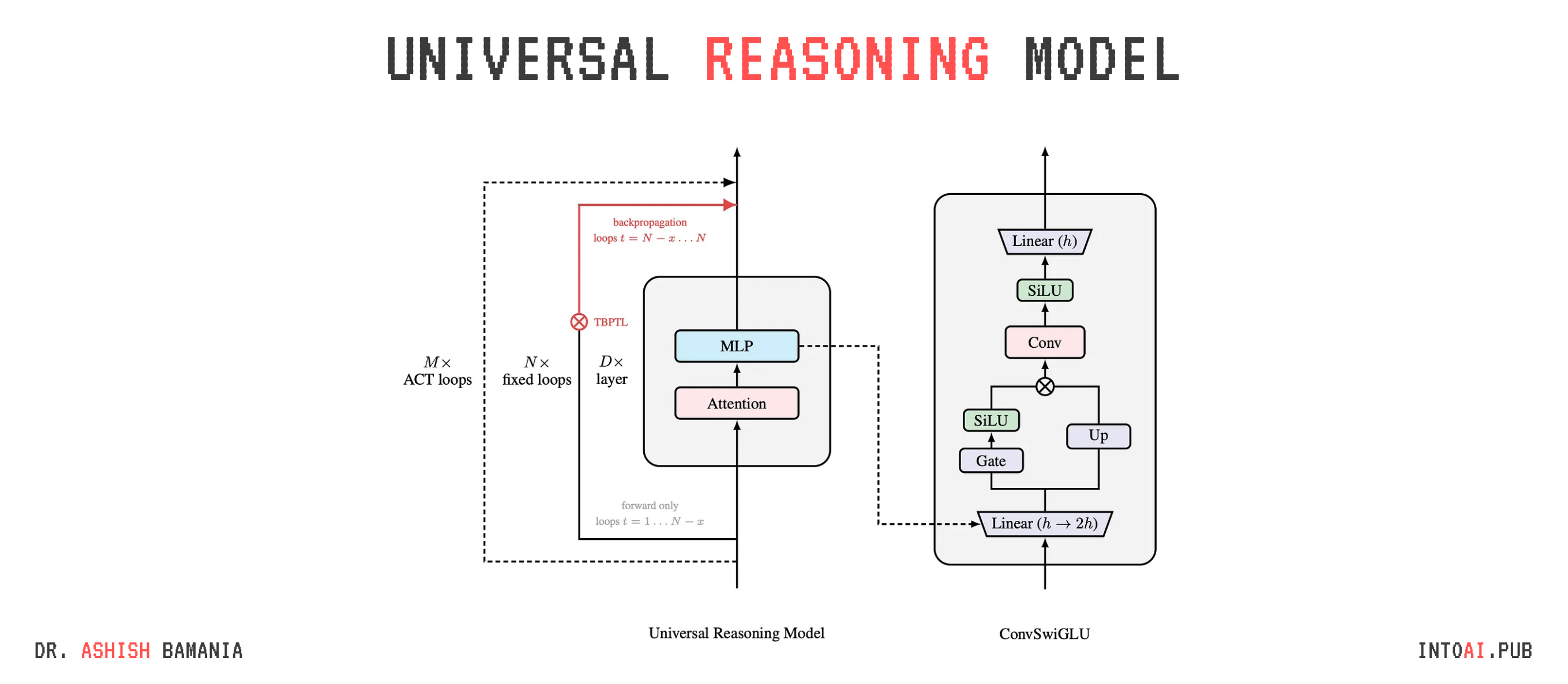
In contrast to the above, ConvSwiGLU applies a depthwise 1D convolution W(dwconv) of kernel size 2 to the tokens as follows, where σ is the SiLU activation function.

The final output from here on is computed by applying W(down) as follows:

By inserting a short depthwise convolution into SwiGLU, ConvSwiGLU allows local token interactions within the FFN. This improves the capacity for nonlinear representation in the URM without adding high computational cost.
The complete URM architecture is shown below, along with the expanded ConvSwiGLU module.
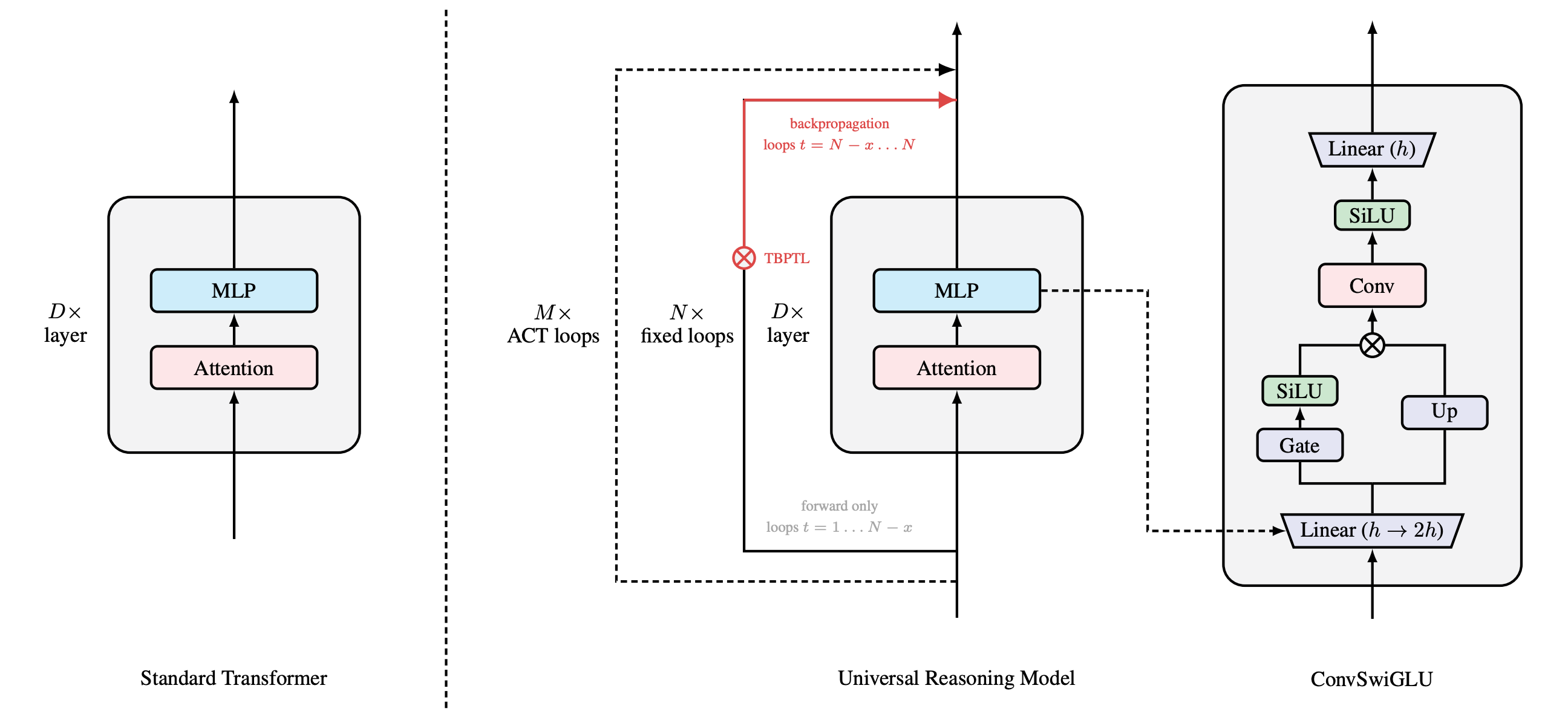
There’s the “TBPTL” shown in red in the illustration above. Let’s discuss this in the next section.
2. Truncated Backpropagation Through Loops (TBPTL)
A URM not only has multiple layers but also uses multiple recurrent loops/ timesteps to reason.
Gradients from very early loops can be noisy, and as the number of loops increases, long gradient chains become unstable, making optimization hard.
This is what TBPTL addresses by:
Treating early loops as forward-only refinement steps, and
Restricting gradient computation to only the later reasoning loops
(If you’re familiar with RNNs, this is an issue that they face as well when training on long sequences. Truncated backpropagation through time (TBPTT) is how they address it.)
For a D-layer URM, that loops for M reasoning steps during training, the recurrent computation is represented as:

where:
h(d)(t)is the hidden state at layerdand reasoning timestepth(d-1)(t)is the input from the previous layer in the same reasoning timesteph(d)(t-1)is the input from the previous reasoning timestep in the same layerF(d)(θ)is the Transformer block at layerd
Instead of backpropagating through all M loops, URM performs:
Forward pass only, for the first
NloopsBoth forward and backward passes for the latter loops (
M - N)

This means that gradients are not propagated through the early loops. This is why the algorithm is called “Truncated” Backpropagation Through Loops.
Instead of computing loss only at the final loop, URM sums losses over all (M − N) loops as follows:

where:
h(D)(t)is the output of the final layer at the reasoning looptyis the targetLrepresents the cross-entropy loss function
The gradients with respect to θ are therefore:

Show Me The Performance
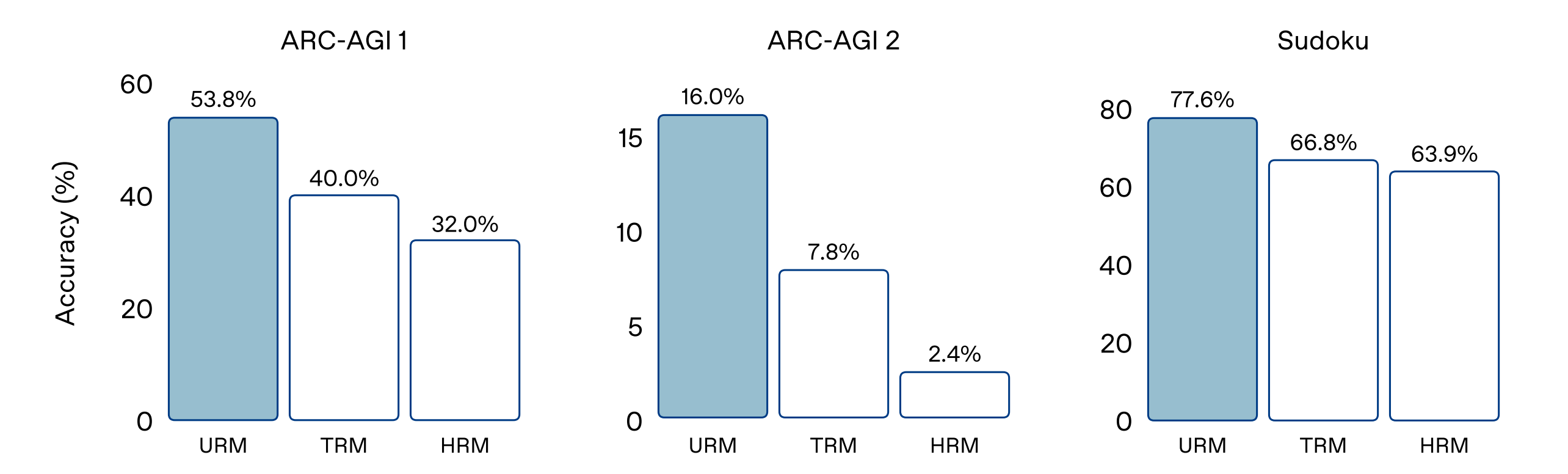
The Universal Reasoning Model (URM) outperforms previous recursive reasoning models by a large margin across all ARC-AGI and Sudoku benchmarks.
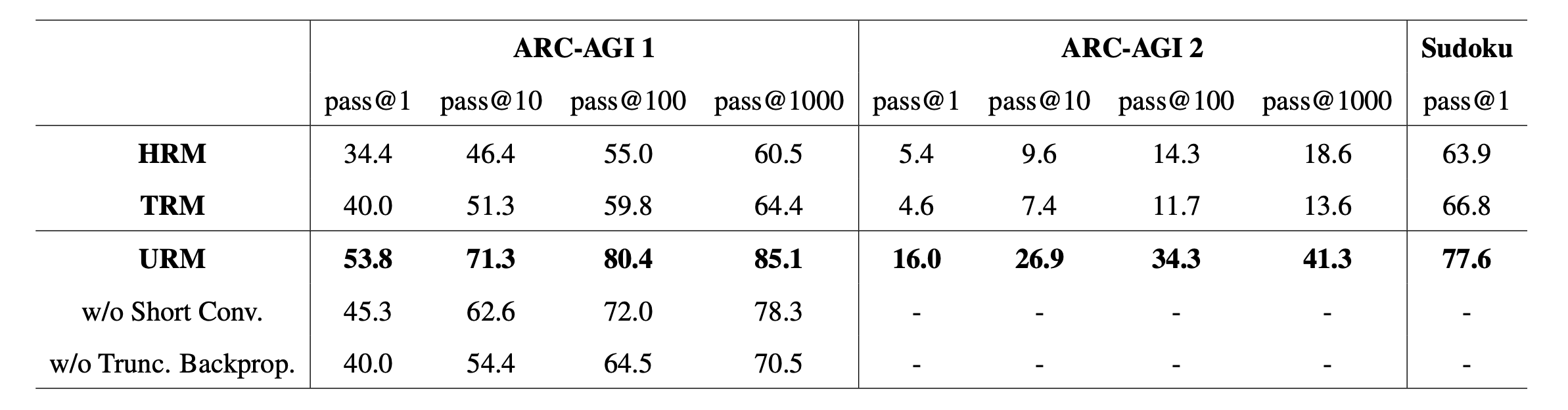
On ARC-AGI 1: URM reaches 53.8% pass@1, compared to 40% (TRM) and 34.4% (HRM)
On ARC-AGI 2: URM achieves 16% pass@1, which is more than 3× TRM and HRM
On Sudoku: URM reaches 77.6% accuracy, surpassing both baselines
What Makes URM Perform So Well?
It seems that sophisticated architectural designs (such as those of HRM/ TRM) do not really improve reasoning performance.
5 learnings from the amazing performance of URMs are:
Recurrent computation with shared parameters is more effective than adding more layers for reasoning tasks.
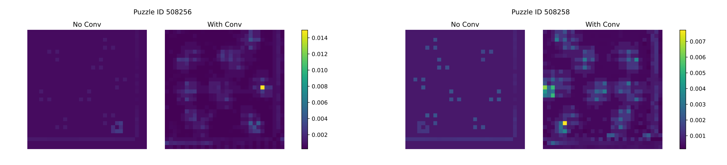
Adding ConvSwiGLU to the MLP leads to richer attention patterns, even though the convolution is applied outside the attention mechanism.
Truncated backpropagation through loops ensures that noisy gradients from early reasoning steps are not used for training, making optimization more stable.
Muon optimizer leads to faster convergence, improving the training efficiency of URMs
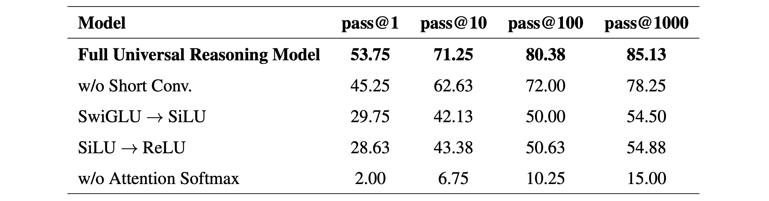
Non-linearity is the real driver of URM’s performance. Removing convolution, SwiGLU, or Attention softmax all lead to a strong performance collapse.
Further Reading
ArXiv research paper titled ‘Universal Reasoning Model’
ArXiv research paper titled ‘Universal Transformers‘
ArXiv research paper titled ‘Adaptive Computation Time for Recurrent Neural Networks‘
If you want to get even more value from this publication and support me in writing these in-depth articles, consider becoming a paid subscriber.
You can also check out my books on Gumroad and connect with me on LinkedIn to stay in touch.